Transcription
PREDICTING THE MARKET POTENTIAL OF PLUG-IN ELECTRIC VEHICLESUSING MULTIDAY GPS DATAMobashwir KhanThe University of Texas at Austin1.120. Cockrell Jr. HallAustin, TX 78712-1076mobashwir@gmail.comKara M. Kockelman(Corresponding author)Professor and William J. Murray Jr. FellowDepartment of Civil, Architectural and Environmental EngineeringThe University of Texas at Austin6.9 E. Cockrell Jr. HallAustin, TX 78712-1076kkockelm@mail.utexas.eduPhone: 512-471-0210The following paper is a pre-print and the final publication can be found inEnergy Policy 46: 225-233, 2012.Presented at the Transportation Research Board’s 91st Annual Meeting, January 2012ABSTRACTGPS data for a year’s worth of travel by 255 Seattle households illuminate how plug-in electricvehicles can match household needs. The results suggest that a battery-electric vehicle (BEV)with 100 miles of range should meet the needs of 50% of one-vehicle households and 80% ofmultiple-vehicle households, when charging once a day and relying on another vehicle or modejust 4 days a year. Moreover, the average one-vehicle Seattle household uses each vehicle 23miles per day and should be able to electrify close to 80% of its miles using a plug-in hybridelectric vehicle (PHEV) with 40-mile all-electric-range. Households owning two or morevehicles can electrify 50 to 70% of their miles using a PHEV40, depending on how they assignthe vehicle across drivers each day. Cost comparisons between the average single-vehiclehousehold owning a Chevrolet Cruze versus a Volt PHEV suggest that when gas prices are 3.50per gallon and electricity rates at 11.2 ct per kWh, the Volt will save the household 535 per yearin operating costs. Similarly, the Toyota Prius PHEV will provide an annual savings of 538 peryear over the Corolla.Key words: Plug-in Electric Vehicles, Battery-electric Vehicles, Long-Term Vehicle UseBACKGROUNDEnergy-security concerns, the rising cost of petroleum, and climate change considerations makeplug-in electric vehicles (PEVs) an intriguing alternative to conventional internal combustionengine (ICE) vehicles. PEVs run partially or fully on electric power from an externally chargedbattery. PEVs include battery-electric vehicles (BEVs) and plug-in hybrid electric vehicles1
(PHEVs). BEVs are driven by an electric motor while PHEVs include an ICE for conventionalpower as needed. PHEVs can function in different modes and different configurations. Readersare referred to Vyas and Santini (2009) for details of different PEV technologies and to Taylor(2009) for a detailed comparison of BEVs and PHEVs. PHEVs are usually denoted by PHEVx,where x refers to the vehicle’s all-electric range (AER). The AER is the distance the vehicle isable to travel purely on electricity under average driving conditions.PEV technology tends to be more expensive than ICE technology because of the high cost ofbatteries. Until recently, a BEV with an AER of 100 miles was estimated to cost themanufacturer at least 16,000 more than a comparable conventional vehicle (Sperling and Lutsey2009, and Frost and Sullivan 2009a), and a PHEV20 and PHEV40 were estimated to cost 8,000and 11,000 more, respectively (Simpson 2006). While such costs are generally falling, evendifferences of 5,000 make electric vehicles less accessible to cost-sensitive customers.Although many governments now provide financial and non-financial incentives to earlyadopters, the observed cost differences remain high. In addition, there are uncertainties ofbattery-replacement costs, energy savings and resale value. Currently, the U.S. governmentprovides an income tax rebate of up to 7,500 per vehicle (depending on the battery size), andCalifornia buyers can receive another 5,000 from the Clean Vehicle Rebates Project (Center forSustainable Energy 2011).The benefits of switching to PEVs are many, including greater energy-security, as nations canreduce reliance on foreign sources of oil (Fontaine 2008, Greene 2010a). PEVs should alsoreduce green-house gas (GHG) emissions in most settings (Kintner-Mayer et. al. 2007, Samarasand Meisterling 2008, and Sioshansi and Denholm 2009) and shift other emissions away frompolluted urban centers by reducing (or eliminating) tailpipe emissions (Thomas 2009, Duvall andKnipping 2007). The 2010 Chevy Volt is rated by the U.S. Environmental Protection Agency(EPA) to travel 93 miles per gallon of equivalent electricity (with one gallon of gasoline ratedequivalent to 33 kW-hr of electricity). In fact, the higher purchase price of electric vehicles maybe recovered over several years of operation. For example, Tuttle and Kockelman (2012) showedhow the net cost of a Nissan Leaf BEV compared to a similarly sized conventional Nissan Versadrops to 250 within ten years of operation at gasoline and electricity prices of 3.00 per gallonand 11.75 ct per kWh, respectively. Simpson (2006) and Lemoine et al. (2008) concluded thathigher gasoline prices and lower manufacturing costs of batteries are key to making PEVseconomically feasible in the long run.One of the biggest hurdles to BEV adoption is “range anxiety”, where owners worry about beingstranded roadside with a fully discharged battery (Tate et. al. 2008, TEP 2011). Higher AERsreduce range anxiety, but at the expense of higher manufacturing costs. AER is also importantfor PHEV owners since it determines the percentage of miles that are electrified, therebyimpacting fuel cost savings. Manufacturers need to know what AERs are most suitable fordifferent consumer markets.This paper addresses such questions. For the manufacturers, it suggests what percentage of theU.S. market may be well-served under multiple AER scenarios (for BEVs and PHEVs). Forconsumers, it tackles questions like: What percentage of driving days can be accommodatedusing BEVs of certain AERs? What percentage of miles will be electrified under different PHEV2
design scenarios? And what savings can households expect in the long run? Honest answers tosuch questions may allow manufactures and consumers to overcome various concerns they haveand pursue a PEV future.Vyas and Santini (2009) sought to address similar questions by relying on the United States 1day National Household Travel Survey (NHTS) data from 2001. Gonder et al. (2007) used oneday GPS data from St. Louis driving to predict gasoline savings under PHEV20 and PHEV40scenarios and concluded that GPS data significantly enhance results, since analysts can discerndetailed driving profiles that affect fuel consumption. They estimated that PHEVs can reduce avehicle’s fuel consumption by roughly 50% compared to conventional vehicles. More recently,Pearre et al. (2011) analyzed multi-day GPS data over a full year from 484 instrumented vehiclesin Atlanta, Georgia. Their results suggest that a substantial fraction of the sampled fleet (32%)may be able to switch to 100-mile AER BEVs if they are willing to adjust driving patterns just 6days a year.Both Vyas and Santini (2009) and Gonder et al. (2007) focused on PHEVs and used one-daydata sets. This research uses GPS data over a one-year period, but from the Seattle area andexamines both PHEV and BEV adoption scenarios. It also estimates annual cost savings forsingle-vehicle households who are willing to switch to a PEV. In addition, the sample isweighted to reflect the Seattle population and single- and multiple-vehicle households areanalyzed separately, since multiple-vehicle households have added flexibility when switchingjust one of their vehicles to a PEV. The goal is to describe PEV adoption rates in light of travelbehavior patterns and household types.The rest of the paper is organized as follows: first, key characteristics of present and forthcomingPEVs are described, so readers are familiar with purchase options. Then, the long-term Seattledriving data are discussed, along with a brief explanation of the merits of using multi-day data.These data are analyzed to determine reasonable adoption and use profiles and ownership costimplications along with utility factors.CURRENT AND UPCOMING PEVsThe Tesla Roadster (a BEV) has sold more than 1500 units in 30 countries since its 2008 release(Gordon-Bloomfield 2011), and the Chevrolet Volt and Nissan Leaf began limited sales in selectUS cities in 2010 (EV Project 2011). Several other PEVs from a broad array of manufacturersare scheduled to enter the market soon. These include different types of vehicles such as the2012 Ford Escape PHEV, which is a sports utility vehicle (SUV) (Plug In America 2011), andthe Dodge Ram, which is a pickup truck (Automotive News 2011). Apart from vehicle type andseating capacity, two critical attributes are battery capacity and range. While the total range of aPHEV is much more than its AER, the AER determines the owner’s likely operating cost savings,petroleum avoidance, and emissions impact. According to Tuttle and Kockelman (2012),expected BEVs tend to have AERs between 60 and 300 miles, while expected PHEVs haveAERs between 10 and 80 miles.The 2011 Chevrolet Volt PHEV is a four-door sedan with a manufacturer suggested retail price(MSRP) of 32,780 after a 7,500 of tax rebate provided by the U.S. government (Chevrolet3
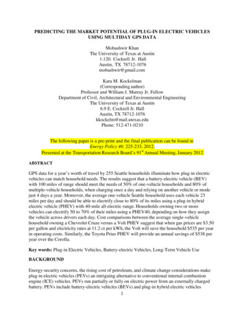
2011). It has a battery size of 16 kWh, and the U.S. EPA has rated it to have an AER of 35 milesunder average driving conditions (EPA 2011). A close ICE counterpart of the Chevrolet Volt isthe 2011 Chevrolet Cruze, which has an MSRP of 16,525 (Chevrolet 2011). The Toyota PriusPHEV, scheduled for release in 2012, is speculated to have an MSRP of 33,500 after a federal 2,500 tax rebate (USA TODAY 2010). Its battery pack is smaller than the Chevrolet Volt, atonly 5.2 kWh and will provide an AER of only 13 miles (Plug In America 2011). The FordEscape PHEV is expected to be released into the market in 2012; it is an SUV with ananticipated AER of 40 miles (Plug In America 2011).Several manufacturers are (or will be) offering BEVs for customers. The 2009 Tesla Roadster isa two-door sports car with a 53kWh battery and an AER of 245 miles (Tesla 2011). After aneligible 7,500 tax rebate, its 101,500 price remains substantial. A more affordable BEV is the2011 Nissan Leaf, a four-door hatchback with a battery size of 24kWh and an EPA-rated AER of73 miles (Nissan 2011, EPA 2011). The Nissan Leaf has an MSRP of 25,280 after an eligible 7,500 tax rebate (Nissan 2011). A close ICE equivalent to the Nissan Leaf is the 2011 NissanVersa 1.8L hatchback, which has an MSRP of 17,410 (Nissan 2011). Other popularmanufacturers, such as BMW, Mercedes, Honda and Toyota, have released or are releasing theirown BEVs (Plug In America 2011).DATA DESCRIPTIONThe data were obtained from the Puget Sound Regional Council’s (PSRC) 2007 Traffic ChoicesStudy across 264 households (and their 445 vehicles) residing in King, Kitsap, Pierce andSnohomish counties of Washington State. The data was collected between November 2004 andApril 2006 using in-vehicle GPS devices and was provided through the National RenewableEnergy Laboratory’s (NREL) Secure Transportation Data Project. Due to the sensitive nature ofthe GPS data and privacy constraints, access to household demographics and vehicle locationswas not feasible. Nevertheless, this rich data set includes lengths and trip durations for eachvehicle at all times of each day over an extended period of time. In addition, householdcharacteristics such as income and vehicle ownership levels are reported, as shown in Table 1.Figure1 illustrates one vehicle’s daily-VMT information over 365 days, as extracted from thedata set.4
Distance Travelled 1271301331361Figure 1 GPS Data Representation of Daily VMT for a Single Sampled VehicleTravel patterns of individuals vary substantially over time, which is why multi-day data, asopposed to conventional single-day data, can provide better insights into travel behavior(Pendyala and Pas 2000). Although the number of households surveyed in these data is relativelysmall, Stopher et al. (2008) showed how the required sample size to attain meaningful results canbe significantly reduced in the case of multiday surveys. Hence, these data may characterize thetravel behavior of metropolitan Seattle households rather well, once corrected for sample biases.To better represent the study area population, each sampled household was weighted using theAmerican Community Survey (ACS) microdata sample for the PSRC’s four counties using thepopulation shares matched on number of vehicles, home-ownership status, and annual householdincome.Descriptive statistics of the unweighted data along with some statistics from Seattle’s AmericanCommunity Survey are shown in Table 1. The average number of drivers and vehicles are 1.63per household in the PSRC data, compared to 2.04 in the ACS data. The average householdincome is clearly lower at 46,658 per year compared to 81,533 per year in the ACS data. Theaverage age of the sampled drivers is about 45 years, which is somewhat older than the region’s39; and a majority of these (60%) are females, compared to 51% for the region. Most of therespondents are fully or partially employed (81%) and the rest of them are home-makers (10%),students (6%) or unemployed (3%).The data set contains 269,357 trip records where the average trip is about 16 miles. These triprecords correspond to 143,004 vehicle-days of data where each vehicle-day implies a day’sworth of data for one vehicle. While the average Seattle trip length of 15.5 miles, as captured bythe GPS device and coded into the data set by the data managers, appears as significantly longerthan the U.S. average of 10.1 (from the 2009 National Household Travel Survey [NHTS]), thedaily VMT is somewhat lower, at 25.4 miles, versus 29.0. Of course, these are unweightedstatistics, to show the biases in the sample. Weighting, which is used on all values presented5
from here forward (including estimated shares of households able to switch to a PEV), offsetsthese to a significant degree.Table 1 Data Set Description (Unweighted)VariableHousehold records (N 255)Number of driversNumber of vehiclesOwn home indicatorRented home indicatorNumber of kidsHousehold income ( /year)Driver records (N 419)Age (years)Female IndicatorEducation (years)Full-time employment statusStd.Maximum 45412.336689.1342.029.0Trip records (N 269,357)VMT per trip (miles)Drive time per trip (minutes)Vehicle-day records (N 143,004)Number of days per vehicleVMT per day (miles)SeattleACSAverage2.040.730.2781,533Some of the cases were not usable due to missing values, inconsistency in reporting, very shortseries of daily-use records and/or nonsensical values. These observations were dropped. Inaddition, zero-VMT days had to be synthesized since the data set did not report any travel whenthe instrumented car was not driven. It was assumed that whenever a vehicle did not report anytravel on a given day, it did not travel that day. The final data set consisted of 255 households,424 vehicles and 419 drivers over 143,004 vehicle-days; thus, there was an average of 341 daysof useful data per vehicle.DATA ANALYSISThe population-corrected data were analyzed to determine which households might reasonablyreplace an existing vehicle with a PEV. Households were divided into single-vehicle householdsand multiple-vehicle households and then divided further, into six cases total, as shown in Figure6
2. Cases 1 and 2 are for single-vehicle households replacing their car with a BEV or a PHEV,respectively.The multiple-vehicle household scenario is more complex. Cases 3 and 4 are for multiple-vehiclehouseholds swapping one of their vehicles with a BEV, and cases 5 and 6 are for PHEVs. In case3 the household replaces the vehicle that travels fewer miles on average with a BEV and thenuses a BEV for all travel made by that vehicle. In case 4, the household replaces any of itsexisting vehicles, and then uses a BEV to meet travel needs of the driver that travels fewer mileseach day, on a day-to-day basis. Of course, all BEV owners will not always know in advancehow far they will need to drive their vehicles each day. So these two assignment-to-driver cases(3 and 4) present the extreme assignment examples, and actual shares (of days covered by aBEV’s range) presumably will lie somewhere between their two percentages.PHEVs do not have any special range limitations (relative to ICEs) and can quickly refuel at gasstations on long trips. To maximize a household’s use of electric power, PHEVs may be assignedto a household’s longer daily drives. Cases 5 and 6 involve the use of the PHEV by the higherVMT vehicle in the household – as estimated on average (Case 5) or on a day-to-day basis (Case6). These two cases also are meant to capture the two extremes of vehicle assignment, and actualshares (of electrified miles) will lie somewhere in between. (Of course, PEV owners can also recharge more than once a day, increasing the percentages further.)Two key questions are tackled under these six cases, as shown in Figure 2. For BEV owners, thepercentage of days that can be covered by the household’s BEV is anticipated (Cases 1, 3 and 4).For PHEV owners, the percentage of household miles that are electrified under differentscenarios is predicted (Cases 2, 5 and 6).HouseholdSingle‐vehiclehouseholdSwitch to a BEV(Case 1)What percentageof days arecovered?Mutliple‐vehiclehouseholdSwitch to a PHEV(Case 2)What percentageof miles areelectrified?Switch a vehicle toa BEVSwitch a vehicle toa PHEVWhich vehicle toswitch?Which vehicle toswitch?The vehicle thattravels less onaverage (Case 3)The vehicle thattravels less on anygiven day (Case 4)What percentageof days arecovered?What percentageof days arecovered?The vehicle thattravels more onaverage (Case 5)What percentageof miles areelectrified?Figure 2 PEV Assignment to Seattle Households7The vehicle thattravels more on anygiven day (Case 6)What percentageof miles areelectrified?
Percentage of Days Covered Using a BEVIf the AER of a BEV is more than the total miles driven by a Seattle vehicle on a given day, thatday is “covered” by the BEV. For each replaced vehicle, the number of days that can be coveredusing a BEV is divided by the number of days in the household’s data series to find the share ofdays whose travel needs can be met by the adjusted fleet. It is assumed that a household is likelyto switch to a BEV if a high percentage of days can be covered when owning a BEV. Since theminimum target on travel-met days is not known and likely to vary from household to household,two extreme values (90% and 99%) and a midpoint value (95%) were used here, assuming thatthis range should capture the preferences and needs of the great majority of vehicle-owninghouseholds. For the small share of longer trips that cannot be covered by a BEV, somehouseholds would be able to charge their cars mid-trip, use rental cars or swap vehicles or modesfor a day or more. The percentage of days that can be covered using a BEV was calculated foreach household.The (population-corrected) shares of Seattle households that can replace a vehicle under each ofthese three percentage values (90, 95 and 99%) were calculated. The method was repeated forBEVs of different AERs, and plots of household percentages (three different plots correspondingto 90, 95 and 99%). Figures 3, 5 and 6 depict the three cases (1, 3 and 4) of BEV adoption.Percentage of Miles Electrified using a PHEVIf a PHEV’s AER exceeds the miles travelled on a given day, all miles were assumed to beelectrified. If not, just the AER portion of miles was assumed electrified. The number of mileselectrified each day for each vehicle was used to determine the percentage of miles electrified foreach replacement PHEV (over the period of each household’s data). The mean of thesepercentages is used as an indication of the share of miles that can be electrified at that AER. Themethod was repeated for different PHEV AERs, and a plot of electrified miles against AERs wascreated. For multiple-vehicle households, the percentage of total household miles electrified wasplotted (instead of the percentage of the PHEV’s miles). Figures 4 and 7 show the plotscorresponding to PHEV adoption as outlined in cases 2, 5 and 6. The results of these calculationsare discussed below.RESULTSThe two cases involving single-vehicle households are discussed first below followed by the fourcases involving multiple-vehicle households.Case 1: Single-vehicle Households Switching to a BEVFor the single-vehicle households two plots are provided. Figure 3 shows how the percentage ofSeattle’s single-vehicle households that can replace their existing vehicle with a BEV variesacross AER levels. The analysis was done for AERs of 60, 70, 80, 90, 100 and 120 miles andquadratic least-squares regression lines are shown.8
90% of days95% of days99% of days100%90%80%% of Households70%60%50%40%30%20%10%0%5060708090100All Electric Range (AER), in miles110120130Figure 3 Maximum Possible Single-vehicle Household Adoption Rates for BEVs in Seattle(Case 1)The dashed line suggests how household adoption rates may vary if households switched toBEVs assuming just 90% or more days in a year must be met by the BEV’s AER. The resultssuggest that BEVs with AERs as low as 60 miles would meet 80% of Seattle’s one-vehiclehouseholds’ travel needs. This is a very relaxed case and will be unrealistic for households whodo not want to rely on other forms of transportation 10% of the time, or 37 days a year.Ideally, households would be willing to switch if all of their travel needs can be met by a BEV.The 99% case is more compelling since it implies that the household will need to find some othermeans of transportation just 4 days a year. The 99% case is shown in the dotted line. As can beseen from the plot, the percentage of single-vehicle households able to meet 99% of their days’travel needs drops significantly across AERs. At an AER of 90 miles, only 40% of the Seattle’ssingle-vehicle households appear able to switch.Finally, the solid line shows the 95% case, where households would have to rely on some othervehicle for transportation about18 days a year. The 95% and 90% cases suggest that there isample opportunity in the Seattle and U.S. markets for regular reliance on BEVs with 60 mileAERs – even in households with just one vehicle – far more than current adoption predictions.For example, microsimulations of Austin households by Musti and Kockelman (2009) suggestjust a 19% fleet composition of PHEVs plus HEVs within 25-years. Similar microsimulations byPaul et al. (2011) for the U.S. market suggest a PHEV fleet share of 3.31% over a 25-yearhorizon when gas prices are held high ( 5.00/gallon) and PHEV prices are relatively low. In9
reality, no one knows what the future will hold, due to uncertainty in innovations, fuel prices,government regulation, and consumer motivation.Case 2: Single-vehicle Households Switching to a PHEVFigure 4 shows how share of electrified miles may vary with AER for single-vehicle householdsif they replace their existing vehicle with a PHEV. The single-vehicle households are dividedinto three categories based on their daily VMT, with cut points of 15 and 30 miles per day. Theweighted-average single-vehicle household’s daily VMT in the Seattle region is 23.4 miles perday.The analysis was performed for AERs of 10, 20, 40 and 60 miles and a logarithmic fit wasapplied for the trend line (since it provided the best fit). Vehicles that travel less on average areable to electrify more of their miles since they stay within or around the AER on more days.Households averaging 15 VMT/daybetween 15 and 30 VMT/dayover 30 VMT/day100%90%VMT Share l Electric Range (AER), in Miles6070Figure 4 Share of VMT Electrified Using PHEVs in Single-vehicle Seattle Households(Case 2)The results suggest that single-vehicle Seattle households that travel (on average) less than 15miles per day can hope to electrify more than 90% of their miles with a PHEV60. A PHEV10,like the forthcoming Toyota Prius, which is less expensive, can electrify close to 50% of its milesif charged just once a day. The Chevrolet Volt has an AER of 35 miles, and should allow formore than 70% electrified miles in single-vehicle households that travel (on average) between 15and 30 miles per day. Single-vehicle households that travel on average more than 30 miles perday would require a PHEV25 to electrify at least 50% of their miles. Since single-vehicle10
households in the Seattle region travel 23 miles per day, to achieve at least 70% electrification, aPHEV of AER around 32 miles would be needed. Since the 2009 NHTS suggests that theaverage U.S. vehicle travels 29 miles/day (Table 1), the average single-vehicle U.S. householdpresumably will require a somewhat higher AER to achieve 70% electrification.Cases 3 and 4: Multiple-vehicle Household Adopting a BEVSimilar analyses to determine the maximum possible BEV adoption rates were performed formultiple-vehicle households. Figures 5 and 6 show the percentage of multiple-vehiclehouseholds that can replace one of their existing vehicles with a BEV. The analysis was done forAERs of 40, 50, 60, 70, 80, 90, 100 and 120 miles and a quadratic function was used for theleast-squares line.Figure 5 presents the results of Case 3, where the household vehicle that travels less on averageis replaced with a BEV. Figure 6 presents the results of Case 4 where the BEV replaces thevehicle that travels less on a day-to-day basis.90% of days95% of days99% of days100%90%% of 100All Electric Range (AER), in miles110120130Figure 5 Maximum Possible Multiple-vehicle Household BEV Adoption Rates in Seattle,with BEV Replacing the Lower Overall-VMT Vehicle (Case 3)11
90% of days95% of days99% of days100%90%% of 100All Electric Range (AER), in miles110120130Figure 6 Maximum Possible Multiple-vehicle Household BEV Adoption Rates in Seattle,with BEV Replacing the Lower-VMT Vehicle on a Day-to-day Basis (Case 4)A comparison of Figures 5 and 6 suggests that replacing the lower VMT vehicle on a day-to-daybasis with a BEV (as shown in Figure 6) allows multiple-vehicle households to serve far moredays’ travel needs – with 99% of travel days’ itineraries being met in 65% of such householdswith 70 mile AER versus just 28% of household contexts if the lower overall-VMT vehicle isused this way. As expected, these percentages are both higher than in Case 1, for a single-vehiclehousehold with a BEV (which averaged 28%) since multiple-vehicle households have moreflexibility. In reality, many households tend to designate household members and onlyoccasionally swap these among each other. Hence, one might safely assume that the actualpercentage of households that can switch to a BEV lies somewhere in between Figures 5 and 6extreme cases. For example, it can be understood that the actual percentage of multiple-vehiclehouseholds that can switch to a BEV of AER 70 miles lies between 65% and 80%.Cases 5 and 6: Multiple-vehicle Households Adopting a PHEVFigure 7 shows travel miles in multiple-vehicle households that may be electrified using a PHEV(assuming once-a-day charging and two different vehicle-assignment rules [Cases 5 and 6]). Theanalysis was done for AERs of 10, 20, 30, 40, 50 and 60 miles and a quadratic fit forms the line.12
PHEV assigned day-to-dayHighest average-VMT vehicle replaced by PHEV90%% of Household VMT l Electric Range (AER), in miles6070Figure 7 Average Shares of Household Miles Electrified (with Standard Deviations) usingPHEVs in Multiple-vehicle Seattle HouseholdsThe solid line presents the results of Case 5, where the household vehicle that travels more onaverage is replaced by the PHEV. The dashed line presents the results of Case 6, where a PHEVreplaces the vehicle that travels more on a day-to-day basis. As expected, Case 6 offers moreelectrified miles. As noted earlier, the actual share of household miles that are electrified willprobably lie between these two cases. For example, such households can electrify about 50% oftheir household miles under Case 5 and 70% under Case 6. The actual percentage of totalhousehold miles for multiple-vehicle households that can be electrified using a PHEV of AER 40miles would lie between 50% and 70%.COST COMPARISONSIn this section, the monetary costs and benefits of switching to a BEV or a PHEV are estimated,as in Tuttle and Kockelman (2012). The 2010 Chevrolet Volt PHEV is compared to the 2011Chevrolet Cruze, the 2010 Nissan Leaf BEV is compared to the 2011 Nissan Versa hatchback,and the upcoming 2012 Toyota Prius PHEV is compared to the 2011 Toyota Corolla. Since gasprices and electricity rates fluctuate over time and space, five gas-price scenarios ( 2.50, 3.50, 4.50, 5.50 and 6.50 per gallon) and three electricity-rate scenarios were considered in theanalysis. The average electric rate across the U.S. is 11.2 ct/kWh (EIA 2011), so this rate wasused as a base case along with 6.0 ct/kWh and 16.0 ct/kWh. The current cost of electricity inWashington State is 8.0 ct/kWh (EIA 2011). Since the percentage of household miles that are13
electrified is similar for single- and multiple-vehicle households, analyses were performed justfor single-vehicle Seattle households that replace their existing vehicle with a BEV or a PHEV.The vehicles were grouped into three categories based on their average daily VMT, with cutoffpoints at 15 and 30 miles. The calculations neglect any added costs of 220-voltage upgrade (forgarage charging outlets) and other l
year over the Corolla. Key words: Plug-in Electric Vehicles, Battery-electric Vehicles, Long-Term Vehicle Use . BACKGROUND. Energy-security concerns, the rising cost of petroleum, and climate change considerations make plug-in electric vehicles (PEVs) an intriguing alternative to conventional internal combustion engine (ICE) vehicles.


![2 CHAPTER 1 [Topic 1] Coulomb's law, electrostatic field and electric .](/img/52/physics.jpg)
