Transcription
Spatial Data Types:Conceptual Foundation forthe Design and Implementation ofSpatial Database Systems and GISMarkus SchneiderFernUniversität HagenPraktische Informatik IVD-58084 HagenGermanymarkus.schneider@fernuni-hagen.de
AbstractSpatial database systems and Geographic Information Systems as their most important application aimat storing, retrieving, manipulating, querying, and analysing geometric data. Research has shown thatspecial data types are necessary to model geometry and to suitably represent geometric data in database systems. These data types are usually called spatial data types, such as point, line, and region butalso include more complex types like partitions and graphs (networks). Spatial data types provide a fundamental abstraction for modeling the geometric structure of objects in space, their relationships, properties and operations. Their definition is to a large degree responsible for a successful design of spatialdata models and the performance of spatial database systems and exerts a great influence on theexpressive power of spatial query languages. This is true regardless of whether a DBMS uses a relational, complex object, object-oriented, or some other kind of data model. Hence, the definition andimplementation of spatial data types is probably the most fundamental issue in the development of spatial DBMS. Consequently, their understanding is a prerequisite for an effective construction of importantcomponents of a spatial database system (like spatial index structures, optimizers for spatial data, spatial query languages, storage management, and graphical user interfaces) and for a cooperation withextensible DBMS providing spatial type extension packages (like spatial data blades and cartridges).The goal of this tutorial is to present the state of the art in the design and implementation of spatial datatypes. First, we summarize the modeling process for phenomena in space in a three-level model andcategorize the treatment of spatial data types with regard to this model. Then we pose design criteria forthe types and analyse current proposals for them according to these criteria. Furthermore, we classifythe proposed types and the operations defined on them from different perspectives. Our main interest isdirected towards approaches which provide a formal definition of the semantics of spatial data typesand which offer methods for their numerically and topologically robust implementation.Markus Schneider, Tutorial “Spatial Data Types“2
ContentsAbstract. 2Contents . 31 What are Spatial Data Types (SDTs)?. 42 Foundations of Spatial Data Modeling .2.1 What Needs to Be Represented?.2.2 A Three-Level Model forPhenomena in Space .2.3 Design Criteria for ModelingSpatial Data Types .2.4 Closure Properties and GeometricConsistency.2.5 Organizing the Underlying Space:Euclidean Geometry versusDiscrete Geometric Bases.2.6 ADTs in Databases for SupportingData Model Independence .2.7 Integrating Spatial Data Types intoa DBMS Data Model.781011121321223 Spatial Data Models and Type Systems . 243.1 What Has to Be Modeled from anMarkus Schneider, Tutorial “Spatial Data Types”Application Point of View? .3.2 Classification.3.3 Examples of Spatial Type Systemsfor Single Spatial Objects.3.4 Partitions .25274 Formal Definition Methods.4.1 Why do We Need FormalDefinitions? .4.2 Point Set Theory .4.3 Point Set Topology.4.4 Finite Set Theory.4.5 Other Formal Approaches.47284348495152575 Tools for Implementing SDTs: DataStructures and Algorithms . 595.1 Representing SDT Values . 605.2 Implementing Atomic SDTOperations . 626 Other Interesting Issues and ResearchTrends . 646.1 Other Interesting Issues notCovered in this Tutorial . 656.2 Current Research Trends . 66References . 673
1 What are Spatial Data Types (SDTs)?Spatial data types . are special data types needed to model geometry and to suitably representgeometric data in database systems Examples: point, line, region; partitions (maps), graphs (networks) . provide a fundamental abstraction for modeling the geometric structure of objects inspace, their relationships, properties, and operations . are an important part of the data model and the implementation of a spatial DBMSThe definition of SDTs . is to a large degree responsible for a successful design of spatial data models . decisively affects the performance of spatial database systems . exerts a great influence on the expressiveness of spatial query languages . should be independent from the data model used by a DBMSMarkus Schneider, Tutorial “Spatial Data Types“4
Conclusions An understanding of SDTs is a prerequisite for an effective construction of important components of a spatial database system spatial index structures, optimizers for spatial data, spatial query languages,storage management, graphical user interfaces for a cooperation with extensible DBMS providing spatial type extension packages spatial data blades, cartridges The definition and implementation of spatial data types is probably the mostfundamental issue in the development of spatial database systems.Focus of this tutorial: present the state of the art in the design and implementation of spatialdata typesMarkus Schneider, Tutorial “Spatial Data Types“5
Contents of this tutorial2 Foundations of Spatial Data Modeling3 Spatial Data Models and Type Systems4 Formal Definition Methods5 Tools for Implementing SDTs: Data Structures and Algorithms6 Other Interesting Issues and Researchs TrendsTutorial based on the book:Markus Schneider, Spatial Data Types for Database Systems - Finite ResolutionGeometry for Geographic Information Systems, LNCS 1288, Springer Verlag, 1997.Markus Schneider, Tutorial “Spatial Data Types“6
2 Foundations of Spatial Data Modeling2.1What Needs to Be Represented?2.2A Three-Level Model for Phenomena in Space2.3Design Criteria for Modeling Spatial Data Types2.4Closure Properties and Geometric Consistency2.5Organizing the Underlying Space: Euclidean Geometry versus DiscreteGeometric Bases2.6ADTs in Databases for Supporting Data Model Independence2.7Integrating Spatial Data Types into a DBMS Data ModelMarkus Schneider, Tutorial “Spatial Data Types“7
2.1 What Needs to be Represented?Two views of spatial phenomena: objects in space (entity-oriented / feature-based view) vector data, spatial database systems space itself (space-oriented / position-based view) raster data, image database systemsObjects in spacecity Berlin, pop 4000000,., area highway A45, .,route SpaceStatement about every point in space land use maps (“thematic maps”) partitions into states, districts, .We consider: modeling single, self-contained objects modeling spatially related collections of objectsMarkus Schneider, Tutorial “Spatial Data Types“8
Fundamental abstractions for modeling single, self-contained e(location of object in spacebut not its extent relevant)(connections in space,movement through space)(extent of an object relevant)Fundamental abstractions for modeling spatially related collections of objectspartitionSpatially embedded network (graph)land usedistrictswardscountriesspeech areashighwaysrailwaysriverselectricityphoneOthers: nested partitions, digital terrain modelsMarkus Schneider, Tutorial “Spatial Data Types“9
2.2 A Three-Level Model for Phenomena in SpaceStructure objectsStructure types: sets, sequences,partitions, networksStructuremodelingOperations: overlay, shortest pathSpatially-referenced objectspopnameObjectmodelingcityObject types: city, state, riverOperations: lies in: city state,flow: river line)Spatial objectsSpatialmodelingMarkus Schneider, Tutorial “Spatial Data Types“Spatial data types: point, line,polygonOperations: point-in-polygon test,intersection10
2.3 Design Criteria for Modeling Spatial Data itionData modelindependenceDesign ofspatial data typesFinite Resolution,numerical robustness,topological encyMarkus Schneider, Tutorial “Spatial Data Types“11
2.4 Closure Properties and Geometric ConsistencyGeneral definition/structure of spatial objectsapplication-driven requirementsBremenformal requirements Niedersachsen spatial objects must be closed under set operations on the underlying point setsSupport of geometric consistency constraints for spatially related objectsadjacent regionsmeeting lines SDT definition must offer facilities to enforce such consistency contraintsMarkus Schneider, Tutorial “Spatial Data Types“12
2.5 Organizing the Underlying Space: Euclidean Geometry versus Discrete Geometric BasesEuclidean space is continuous (p (x, y) IR2) basis of Computational Geometry algorithmsBut: computer numbers are finite and discrete (p (x, y) real real) numerical rounding errors topological inconsistencies and degeneraciesIs D on A?Is D properly contained in the areabelow A and B?D'DABWhat happens ifthere is a segmentC between D andD'? formal SDT definitions must bear in mind the finite representations available in computersMarkus Schneider, Tutorial “Spatial Data Types“13
Solution: avoid computation of any new intersection points within geometric operationsDefinition ofspatial types and operationsTreatment of numerical problems uponupdates on the geometric basisTwo approaches: Simplicial complexesFrank & Kuhn 1986Egenhofer, Frank & Jackson 1989 RealmsGüting & Schneider 1993Schneider 1997Markus Schneider, Tutorial “Spatial Data Types“14
Simplicial Complexes topological relations are separately recorded and independent of metric positions use of k-simplices for representing minimal spatial objects of dimension k construction rule: k-simplex consists of k 1 simplices of dimension k 1 component of a simplex is called faceetc.0-simplex1-simplex2-simplex3-simplex two completeness principles completeness of incidence: the intersection of two k-simplices is either empty or aface of both simplices no line intersection at points which are not start or end points of the lines, no twogeometric objects may exist at the same location (geometry only recorded once) completeness of inclusion: every k-simplex is a face of a (k 1)-simplex all point are end points of lines, all lines are boundaries of triangles, etc.; noisolated points, no lines which are not part of a boundaryMarkus Schneider, Tutorial “Spatial Data Types“15
Simplicial complex: finite set of simplices such that the intersection of any two simplicesis empty or a facecorrect simplicial complexesno simplicial complexes Advantages maintenance of topological consistency approach fulfils closure properties Drawbacks unfortunately: no spatial algebra has been defined on top of this approach triangulation of space would lead to space-consuming representations of spatialobjects no treatment of numerical problems: additional data structures needed to realize (atleast imprecise) metric operationsMarkus Schneider, Tutorial “Spatial Data Types“16
RealmsCABDRealm (intuitive notion): description of the complete underlying geometry (all points andlines) of an application or application spaceRealm (formally): A finite set of points and non-intersecting line segments defined over agrid such that each point and each end point of a segment is a grid point each end point of a segment is also a point of the realm no realm point lies within a segment any two distinct segments do neither properly intersect nor overlap A realm is a spatially embedded planar graphMarkus Schneider, Tutorial “Spatial Data Types“17
All numerical problems are treated below the realm layer: input: application data that are sets of points and intersecting line segments output: “realmified” data that have become acquainted with each other basic idea: slightly distort/perturb both segmentsD'DBBAAGood solution?Markus Schneider, Tutorial “Spatial Data Types“18
DEAIntersection of segment A withsome further segment CBCObservations Segments can move far awayfrom their original position byiterated intersections! Topological errors can occur:point p is now on the wrongside of A!DpAMarkus Schneider, Tutorial “Spatial Data Types“EBC19
Solution: redrawing of segments within their envelope (Greene & Yao 1986)PSegments are “caught” within theirenvelope can never cross a gridpointAdvantages of the realm concept definition of distinct SDTs on a common domain, guarantee of closure properties protection of geometric computation in query processing from problems of numericalrobustness and topological correctness enforcement of geometric consistency of related spatial objectsDisadvantages of the realm concept no SDT operations possible that create new geometries (leave the realm closure), e.g.,convex hull, voronoi integration of realms into database systems somewhat difficult, propagation of realmupdates to realm-based attribute values in database objectsMarkus Schneider, Tutorial “Spatial Data Types“20
2.6 ADTs in Databases for Supporting Data Model IndependenceModeling aspects Separation of DBMS data model and application-specific data types/algebras Modularity, conceptual clarity Reusability of ADTs for different DBMS data models Extensibility of DBMS data modelsImplementation aspects Modularity, information hiding, exchange of implementations Employment of specialized methods (e.g. Computational Geometry for SDTs) Efficiency of data structures for data types and algorithms for operationsMarkus Schneider, Tutorial “Spatial Data Types“21
2.7 Integrating Spatial Data Types into a DBMS Data ModelIntegration of single, self-contained spatial objects can be realized in a data model independent way ( ADTs) Basic concept: represent “spatial objects” (i.e., points, lines, regions) by objects of theDBMS data model with at least one SDT attribute DBMS data model must be open for new, user-defined types ADT support, data model independence, extensibility Example for the relational model:relation states(sname: string, area: region, spop: integer)relation cities( cname: string, center: point, extent: region,cpop: integer)relation rivers(rname: string, route: line)Markus Schneider, Tutorial “Spatial Data Types“22
Integration of spatially related collections of objects not data model independent partitions set of database objects with region attribute? loss of information: disjointedness or adjacency of regions cannot be modeled Güting 1988: SDT area, but: no support of this integrity constraint by the DBMS networks not much research on spatially embedded networks e.g., Güting 1994: GraphDB with explicit graphs integrated into an OO modelMarkus Schneider, Tutorial “Spatial Data Types“23
3 Spatial Data Models and Type Systems3.1What Has to Be Modeled from an Application Point of View?3.2Classification3.3Examples of Spatial Type Systems for Single Spatial Objects3.4PartitionsMarkus Schneider, Tutorial “Spatial Data Types“24
3.1 What Has to Be Modeled from an Application Point of View?Spatial data types single, self contained objects: points, lines, regions spatially related collections of objects: partitions, networksSpatial operations spatial predicates returning boolean values topological relationshipse.g., equal, unequal, disjoint, adjacent (neighboring), intersect (overlap), meet(touch), inside (in), outside, covered by, contains metric relationshipse.g., in circle, in window spatial order and strict order relationshipse.g., behind / in front of, above / below, over / under, inside / contains directional relationshipse.g., north / south, left / rightMarkus Schneider, Tutorial “Spatial Data Types“25
Spatial Operations (continued) spatial operations returning numberse.g., area, perimeter, length, diameter, dist, mindist, maxdist, direction, components(cardinality) spatial operations returning new spatial objects object construction operationse.g., union, intersection, difference, convex hull, center, boundary (border), box object transformation operationse.g., extend, rotate, translate spatial operations on sets of spatially related objects general operationse.g., voronoi, closest, compose, decompose operations for partitionse.g., overlay, superimposition, fusion, cover, windowing, clipping operations for networkse.g., shortest pathMarkus Schneider, Tutorial “Spatial Data Types“26
3.2 ClassificationConcrete Models point-based models, e.g. Güting 1988 (geo-relational algebra) Worboys & Bofakos 1993 (complex regions with holes) Egenhofer & Herring 1990, Egenhofer & Franzosa 1991, . (topological relationships) Belussi, Bertino & Catania 1997, Grumbach, Rigaux & Segoufin 1998(linear constraint approach) discrete models Güting & Schneider 1995 (ROSE algebra) Frank & Kuhn 1986, Egenhofer, Frank & Jackson 1989 (simplex-based model)Abstract Models logic (pointless, axiomatic) models, e.g. Cui, Cohn & Randell 1993, . (spatial logic)Markus Schneider, Tutorial “Spatial Data Types“27
3.3 Examples of Spatial Type Systems for Single Spatial Objects(1) Güting 1988 (geo-relational algebra)(based on point set theory) Relational algebra viewed as a many-sorted algebra (relations atomic data types) Sorts: rel; int, real, string, bool; point, line, pgon, area example relation: states(sname: string, extent: area, cpop: int) a point value is a single point, a line value is a polyline, a pgon value is a polygonwithout holes special type area for modeling partitions but: partition constraints are not maintained by the system but by the user generalizations: reg {pgon, area}, ext {line, reg}, geo {point, ext}Geometric predicates , :geoi geoi boolinside:geo reg boolintersects:ext ext boolis neighbor of: area area boolMarkus Schneider, Tutorial “Spatial Data Types“insideintersectsis neighbor of28
Geometric relation operationsline* line* point*line* reg* line*pgon* reg* pgon*overlay:area* area* area*vertices:ext* point*voronoi:point* reg area*closest:point* point relintersection:intersectionvoronoiOperations returning atomic geometric objectsconvex hull:point* pgoncenter:point* pointext pointconvex hullMarkus Schneider, Tutorial “Spatial Data Types“center29
Operations returning numbersdist:point point realmindist, maxdist:geo geo realdiameter:point* reallength:line realperimeter, area:reg realComparison to design criteriaRemarks general definition, closure properties formal definition finite precision arithmetic support for geometric consistency( ) efficiency extensibility data model independence Markus Schneider, Tutorial “Spatial Data Types“ only simple polygons no union, difference of polygons forming the intersection of twospatial objects must be embeddedin a relation operation no numerically critical operationsincluded simple data structures algorithms30
(2) Worboys & Bofakos 1993(based on point set topology) complex spatial regions with holes and islands within holes to any finite level atom: subset of IR2 that is topologically equivalent to a closed disc base area: aggregation of atoms whose structure is described by a skeleton graphcConstraintsvbebdvcfvdvagave the intersection of any two distinctatoms is either empty or asingleton setvgvf composite object has no holes generic area: recursive construction of complex spatial regionshhadeae cfgbMarkus Schneider, Tutorial “Spatial Data Types“ cbdfg31
Constraintsacbdge fh for each vertex their successors form a base area for each vertex v root and each successor w of v holds: (a) w v,(b) the intersection of w and the boundary of v has finite cardinality operations: e.g., equals, intersection, union, difference, boundary, adjacent, centroid,area, perimeter, cardinality, components, connectedComparison to design criteria general definition, closure properties formal definition finite precision arithmetic support for geometric consistency efficiency? extensibility? data model independence Markus Schneider, Tutorial “Spatial Data Types“(only for regions)32
(3) Egenhofer & Herring 1990, Egenhofer & Franzosa 1991(based on point set topology) goal: a “complete” collection of topological relationships between two spatial objects topological relationships are invariant under translation, rotation, and scaling originally: topol. relationships between two simple, connected regions without holesAboundary Ainterior A 4-intersection model: 4 intersection sets between boundaries and interiors of twoobjectsExtensions 9-intersection model (Egenhofer 1991): consider also intersections of A and A withthe exterior / complement A ( 92 81 combinations, 8 are valid) include point and line features (Egenhofer & Herring 1992, de Hoop & van Oosterom1992)Markus Schneider, Tutorial “Spatial Data Types“33
4-intersection model A B A B A BA B relationship nameA and B are disjointA contains B / B inside Aequaldisjointcovered by / coversoverlapmeetinside / containsA inside B / B contains AA and B meetA and B are equalA covers B / B covered by AA covered by B / B covers AA and B overlap42 16 combinations, 8 are validMarkus Schneider, Tutorial “Spatial Data Types“34
dimension extended method (Clementini, Felice & van Oosterom 1993): considerdimension of the intersection (empty, 0D, 1D, 2D in 2D space) 44 256 combinations for each relationship group (area / area, line / area, point /area, line / line, point / line, point / point), totally 52 are validtoo many relationships to be remembered!alternative: five basic relationships touch, in, cross, overlap, disjoint plus three operatorsb, f, t to obtain boundariesone can prove: 5 relationships are mutually exclusive 5 relationships plus 3 boundary operators can distinguish all 52 configurations consider regions with holes (Egenhofer, Clementini & Di Felice 1994) consider composite regions (Clementini, Di Felice & Califano 1995)Markus Schneider, Tutorial “Spatial Data Types“35
(4) Belussi, Bertino & Catania 1997, Grumbach, Rigaux & Segoufin 1998(based on a linear constraint approach) basic idea of the spatial constraint model: represent spatial objects finitely as infinitecollections of points satisfying first-order formulas a convex polygon is the intersection of a finite set of half planes, i.e., a conjunction ofthe inequalities defining each half plane a non-convex polygon is the union (logical disjunction) of a finite set of convex polygons(disjunctive normal form (DNF)){(x, y) x 1 x -1 y 1 y -1}{(x, y) y x 0}{(x, y) x -1 y -1 x y 2 0}half plane representationp1p2representation of two convex polygonsDNF repr.:p1 p2convexification of a polygonMarkus Schneider, Tutorial “Spatial Data Types“p1p2polygon with disjoint components36
CHNF (convex with holes normal form) is a generalization of DNFp1p2p4DNF repr.:p3p1 p2 p3 p4q1q2CHNF repr.:q1 q2Comparison to design criteria general definition, closure properties formal definition finite precision arithmetic( ) support for geometric consistency efficiency? extensibility? data model independence Markus Schneider, Tutorial “Spatial Data Types“37
(5) Güting & Schneider 1995 (ROSE algebra)(based on a discrete geometric basis) ROSE RObust Spatial Extension system of realm-based spatial data types (points, lines, regions) whose objects arecomposed of realm elements (points and segments over a discrete geometric domain)a points valuea lines valuea regions value ROSE algebra offers a comprehensive collection of precisely defined operations formanipulating such values, e.g. (let EXT {lines, regions}, GEO {point} EXT) geo, geo1, geo2 GEO, ext, ext1, ext2 EXT, obj OBJinside:geo regions booledge-/vertex-inside:regions regions boolarea-/edge-disjoint:regions regions boolMarkus Schneider, Tutorial “Spatial Data Types“38
ROSE algebra also contains operations which are usually numerically critical, e.g.on border of:points ext boolborder in common:ext1 ext2 boolClosure properties are fulfilled for intersection, union, and difference due to generaldefinition of spatial data typesintersection:points points pointsintersection:lines lines points(no embedding into e.g.intersection:regions regions regionsrelation operations needed)intersection:regions lines linesplus, minus:geo geo geoSpatial operations for manipulating sets of spatially related objects (i.e., databaseobjects) defined by a general “object model interface”sum:set(obj) (obj geo) geoclosest:set(obj) (obj geo1) geo2 set(obj)(also operations for overlay, fusion, and decompose)Markus Schneider, Tutorial “Spatial Data Types“39
Other operationsvertices:ext pointscontour:regions linesinterior:lines regionsno of components:geo intComparison to design criteria general definition, closure properties formal definition finite precision arithmetic support for geometric consistency efficiency extensibility data model independence Markus Schneider, Tutorial “Spatial Data Types“40
(6) Cui, Cohn & Randell 1993(based on logic) pointless approach: regions are the basic entities, no points, no lines axiomatic approach to representing and reasoning about topological spatial data basic binary relation C(x, y): “x connects with y” x C(x, y) xy [C(x, y) C(y, x)]reflexitivity of Csymmetry of C axiomatic formulation of topological relationshipsDC(x, y)P(x, y)x yO(x, y)PO(x, y)EC(x, y)TPP(x, y)NTTP(x, y) def def def def def def def def C(x, y)“x is disconnected from y” z [C(z, x) C(z, y)]“x is a part of y”P(x, y) P(y, x)“x is identical with y” z [P(z, x) P(z, y)]“x overlaps y”O(x, y) P(x, y) P(y, x)“x partially overlaps y”C(x, y) O(x, y)“x is externally connected with y”PP(x, y) z [EC(z, x) EC(z, y)] “x is a tangential proper part of y”PP(x, y) z [EC(z, x) EC(z, y)]“x is a nontangential properpart of y”Markus Schneider, Tutorial “Spatial Data Types“41
topological model to interpret the theory: C(x,y) holds when the topological closures ofregions x and y share a common point similar results like Egenhofer et al.: 8 mutually exhaustive and pairwise disjoint relationsDC (disjoint)EC (meet)PO (overlap) (equal)TPP (covered by / covers)TPP-1 (covers / covered by)NTTP (inside / contains)NTPP-1 (contains / inside)Comparison to design criteria general definition, closure properties formal definition finite precision arithmetic support for geometric consistency efficiency? extensibility? data model independence Markus Schneider, Tutorial “Spatial Data Types“42
3.4 Partitions partition: subdivision of the plane into pairwise disjoint regions where each region isassociated with an attribute having a simple or even complex structure partition implicitly models topological relationships neighborhood of different regions which may have common boundaries disjointedness of different regions (except for boundaries) application-specific operationsoverlay1Markus Schneider, Tutorial “Spatial Data Types“overlay2fusion43
superimpositionwindowdifferenceMarkus Schneider, Tutorial “Spatial Data Types“44
other operations: reclassify, cover, clipping Scholl & Voisard 1989 identification of application-specific operations on maps complex object algebra extended by a data type for regions plus some operations onregions (union, intersection, difference) a map is a set of tuples with a region attribute elementary region: single polygon, region: set of polygons problems: region type not closed under union operation, no control of partitionconstraints through the model, deeply data model dependent Erwig & Schneider 1997 formal definition of spatial partitions basic idea: a partition is a mapping from IR2 to some label type, i.e., regions of apartition are assigned single labels, adjacent regions have different labels in theirinterior, a boundary is assigned the pair of labels of both adjacent regionsMarkus Schneider, Tutorial “Spatial Data Types“45
three powerful operations that are closed under partitions and that are sufficient toexpress all known (generalized) application-specific operationsintersection: compute the geometric intersection of all regions of two partitions andproduce a new spatial partition; each resulting region is assigned the pair oflabels of the original two intersecting regions; labels on the boundaries arederived correspondinglyrelabel: change the labels of the regions of a partition either by renaming the label ofeach region or by mapping distinct labels of two or more regions to a new label;adjacent regions in the result partition are fusedrefine: look with finer granularity on regions and reveal and enumerate the connectedcomponents of regions other approaches: e.g., Frank 1987, Huang, Svensson & Hauska 1992, Tomlin 1990Markus Schneider, Tutorial “Spatial Data Types“46
4 Formal Defini
Markus Schneider, Tutorial "Spatial Data Types" 6 Contents of this tutorial 2 Foundations of Spatial Data Modeling 3 Spatial Data Models and Type Systems 4 Formal Definition Methods 5 Tools for Implementing SDTs: Data Structures and Algorithms 6 Other Interesting Issues and Researchs Trends Tutorial based on the book: