Transcription
1Uintah User GuideJim Guilkey, Todd Harman, Justin Luitjens, John Schmidt, Jeremy Thornock, J. Davisonde St. Germain, Siddharth Shankar, Joseph Peterson, Carson BrownleeUUSCI-2009-007Scientific Computing and Imaging InstituteUniversity of UtahSalt Lake City, UT 84112 USASeptember 15, 2009
Uintah User GuideJim Guilkey, Todd Harman, Justin Luitjens,John Schmidt, Jeremy Thornock, J. Davison de St. Germain,Siddharth Shankar, Joseph Peterson, Carson BrownleeVersion 1.1
Contents1 Overview of Uintah1.1 The Center for the Simulation of AccidentalSAFE) . . . . . . . . . . . . . . . . . . . . .1.1.1 Center History . . . . . . . . . . . .1.2 Uintah Software . . . . . . . . . . . . . . . .1.2.1 Software Ports . . . . . . . . . . . .1.2.2 Uintah Software History . . . . . . .Fires and. . . . . . . . . . . . . . . . . . . . . . . . . .Explosions (C. . . . . . . . . . . . . . . . . . . . . . . . . . . . . . . . . . . . . . . . .2 Using Uintah2.1 Installing the Uintah Software . . . .2.2 Mechanics of Running sus . . . . . .2.3 Uintah Problem Specification (UPS)2.4 Simulation Components . . . . . . .2.5 Time Related Variables . . . . . . . .2.6 Data Archiver . . . . . . . . . . . . .2.7 Simulation Options . . . . . . . . . .2.8 Geometry objects . . . . . . . . . . .2.9 Boundary conditions . . . . . . . . .2.10 Grid specification . . . . . . . . . . .2.11 Regridder . . . . . . . . . . . . . . .2.12 Load Balancer . . . . . . . . . . . . .2.13 UDA . . . . . . . . . . . . . . . . . .3 Visualization tools – VisIt3.1 Reading Uintah Data Archives3.2 Plots . . . . . . . . . . . . . .3.3 Operators . . . . . . . . . . .3.4 Vectors . . . . . . . . . . . . .3.5 AMR datasets . . . . . . . . .3.6 Examples . . . . . . . . . . .3.6.1 Volume visualization .3.6.2 Particle visualization 262629
3.6.33.6.43.6.53.6.63.6.7Visualizing patch boundariesIso-surfaces . . . . . . . . .Streamlines . . . . . . . . .Visualizing extra cells . . .Picking on particles . . . . .4 Data Extraction Tools4.1 puda . . . . . . . . .4.2 partextract . . . . .4.3 lineextract . . . . . .4.4 compute Lnorm udas.5 Arches5.1 Introduction . . . . . . . . . . . . . . . . . . . . . . . . . .5.2 Governing Equations . . . . . . . . . . . . . . . . . . . . .5.2.1 Subgrid Turbulence Models . . . . . . . . . . . . .5.2.2 Subgrid Momentum Dissipation . . . . . . . . . . .5.2.3 LES Algorithm . . . . . . . . . . . . . . . . . . . .5.3 Uintah Specification . . . . . . . . . . . . . . . . . . . . .5.3.1 Basic Inputs . . . . . . . . . . . . . . . . . . . . . .5.3.2 Time Integrator . . . . . . . . . . . . . . . . . . . .5.3.3 Transport Equation Options . . . . . . . . . . . . .5.3.4 Initial and Boundary Conditions . . . . . . . . . . .5.3.5 Turbulence Models . . . . . . . . . . . . . . . . . .5.3.6 Properties, Reaction and Sub-Grid Mixing . . . . .5.3.7 Extra Scalar Solvers . . . . . . . . . . . . . . . . .5.3.8 Additional Transport Equations . . . . . . . . . . .5.3.9 Direct Quadrature Method of Moments (DQMOM)5.4 Examples . . . . . . . . . . . . . . . . . . . . . . . . . . .Almgren MMS . . . . . . . . . . . . . . . . . . . . . . . .Periodic Box Problem . . . . . . . . . . . . . . . . . . . .Helium Plume . . . . . . . . . . . . . . . . . . . . . . . . .Methane Plume . . . . . . . . . . . . . . . . . . . . . . . .Fast Cookoff . . . . . . . . . . . . . . . . . . . . . . . . . .6 ICE6.1 Introduction . . . . . . . . . . . . .6.1.1 Governing Equations . . . .6.2 Algorithm Description . . . . . . .6.3 Uintah Specification . . . . . . . .6.3.1 Basic Inputs . . . . . . . . .6.3.2 Semi-Implicit Pressure 45454545555565658596061.63636366676768
6.46.3.3 Physical Constants . . . . . . . . . . . . . . . .6.3.4 Material Properties . . . . . . . . . . . . . . . .6.3.5 Equation of State . . . . . . . . . . . . . . . . .6.3.6 Exchange Properties . . . . . . . . . . . . . . .6.3.7 BoundaryConditions . . . . . . . . . . . . . . .6.3.8 Output Variable Names . . . . . . . . . . . . .6.3.9 XML tag description . . . . . . . . . . . . . . .Examples . . . . . . . . . . . . . . . . . . . . . . . . .Poiseuille Flow . . . . . . . . . . . . . . . . . . . . . .Combined Couette-Poiseuille Flow . . . . . . . . . . . .Shock Tube . . . . . . . . . . . . . . . . . . . . . . . .Shock Tube with Adaptive Mesh Refinement . . . . . .2D Riemann Problem with Adaptive Mesh RefinementExplosion 2D . . . . . . . . . . . . . . . . . . . . . . .ANFO Rate Stick . . . . . . . . . . . . . . . . . . . . .7 MPM7.1 Introduction . . . . . . . . . . . . . . . . .7.2 Algorithm Description . . . . . . . . . . .7.3 Shape functions for MPM and GIMP . . .7.4 Uintah Implementation . . . . . . . . . . .7.5 Uintah Specification . . . . . . . . . . . .7.6 Examples . . . . . . . . . . . . . . . . . .Taylor Impact Test . . . . . . . . . . . . .Sphere Rolling Down an Inclined Plane . .Crushing a Foam Microstructure . . . . . .Hole in an Elastic Plate . . . . . . . . . .Tungsten Sphere Impacting a Steel Target8 MPMICE8.1 Introduction . . . . . . . . . . . . . . . . .8.2 Theory - Algorithm Description . . . . . .8.3 HE Combustion Models . . . . . . . . . .8.3.1 Simple Burn . . . . . . . . . . . . .8.3.2 Steady Burn . . . . . . . . . . . . .8.3.3 Unsteady Burn . . . . . . . . . . .8.4 Examples . . . . . . . . . . . . . . . . . .Mach 2 Wedge . . . . . . . . . . . . . . . .Cylinder in a Crossflow . . . . . . . . . . .”Cylinder Test” . . . . . . . . . . . . . . .Cylinder Pressurization Using Simple BurnExploding Cylinder Using Steady Burn . 0182184
T-Burner Example Using Unsteady Burn . . . . . . . . . . . . . . . . . 1869 Glossary1904
Chapter 1Overview of Uintah1.11.1.1The Center for the Simulation of AccidentalFires and Explosions (C-SAFE)Center HistoryThe Uintah software suite was created by the Center for the Simulation of AccidentalFires and Explosions (C-SAFE). C-SAFE was originally created at the University ofUtah in 1997 by the Department of Energy’s Accelerated Strategic Computing Initiative’s (ASCI) Academic Strategic Alliance Program (ASAP). (ASCI has since beenrenamed to the Advanced Simulation and Computing (ASC) program.)Center ObjectiveC-SAFE’s primary objective has been to provide a software system in which fundamental chemistry and engineering physics are fully coupled with nonlinear solvers,visualization, and experimental data verification, thereby integrating expertise from awide variety of disciplines. Simulations using the Uintah software can help to betterevaluate the risks and safety issues associated with fires and explosions in accidentsinvolving both hydrocarbon and energetic materials.Target SimulationThe Uintah software system was designed to support the solution of a wide rangeof highly dynamic physical processes using a large number of processors. However,our specific target simulation has been the heating of an explosive device placed in alarge hydrocarbon pool fire and the subsequent deflagration explosion and blast wave(Figure 1.1). The explosive device is a small cylindrical steel container (4” outsidediameter) filled with plastic bonded explosive (PBX-9501). Convective and radiativeheat fluxes from the fire heat the outside of the container and subsequently the PBX.5
After some amount of time the critical temperature in the PBX is reached and theexplosive begins to rapidly decompose into a gas. The solid-¿gas reaction pressurizesthe interior of the steel container causing the shell to rapidly expand and eventuallyrupture. The gaseous products of reaction form a blast wave that expands outwardalong with pieces of the container and any unreacted PBX. The physical processesin this simulation have a wide range in time and length scales from microsecondsand microns to minutes and meters. Uintah was designed as a general-purpose fluidstructure interaction code that can simulate not only this scenario but a wide range ofrelated problems.Complex simulations suchas this require both immensecomputational power andcomplex software. Typicalsimulations include solversfor structural mechanics, fluids, chemical reactions, andmaterial models.All ofthese aspects must be integrated in an efficient mannerto achieve the scalability required to perform these simulations. The heart of Uintah is a sophisticated computational framework thatcan integrate multiple simulation components, analyzethe dependencies and communication patterns betweenthem, and efficiently execute the resulting multiphysics simulation. Uintahalso provides mechanisms forautomating load-balancing,checkpoint/restart, and parallel I/O. The Uintah corewas designed to be general,Target Simulation - Fire-Containerand is appropriate for use in Figure 1.1:Explosion.a wide range of PDE algorithms based on structured(adaptive) grids and particle-in-cell algorithms.6
1.2Uintah SoftwareThe Uintah Computational Framework (also referred to as Uintah or the UCF) consistsof a set of software components and libraries that facilitate the solution of PartialDifferential Equations (PDEs) on Structured AMR (SAMR) grids using up to hundredsto thousands of processors.One of the challenges in designing a parallel, component-based and multi-physicsapplication is determining how to efficiently decompose the problem domain. Components, by definition, make local decisions. Yet parallel efficiency is only obtainedthrough a globally optimal domain decomposition and scheduling of computationaltasks. Typical techniques include allocating disjoint sets of processing resources to eachcomponent, or defining a single domain decomposition that is a compromise betweenthe ideal load balance of multiple components. However, neither of these techniqueswill achieve maximum efficiency for complex multi-physics problems.Uintah uses a non-traditional approach to achieving parallelism by employing anabstract task graph representation to describe computation and communication. Thetask graph is an explicit representation of the computation and communication that occur in the coarse of a single iteration of the simulation (typically a timestep or nonlinearsolver iteration). Uintah components delegate decisions about parallelism to a scheduler component by using variable dependencies to describe communication patternsand characterizing computational workloads to facilitate a global resource optimization. The task graph representation has a number of advantages, including efficientfine-grained coupling of multi-physics components, flexible load balancing mechanismsand a separation of application concerns from parallelism concerns. However, it createsa challenge for scalability which we overcome by creating an implicit definition of thisgraph and representing it in a distributed fashion.The primary advantage of a component-based approach is that it facilitates the separate development of simulation algorithms, models, and infrastructure. Componentsof the simulation can evolve independently. The component-based architecture allowspieces of the system to be implemented in a rudimentary form at first and then evolveas the technologies mature. Most importantly, Uintah allows the aspects of parallelism(schedulers, load-balancers, parallel input/output, and so forth) to evolve independently of the simulation components. Furthermore, components enable replacement ofcomputation pieces without complex decision logic in the code itself.Please see the Developers Guide hAPI.pdf) for more information about the internal architecture of Uintah.1.2.1Software PortsUintah has been ported and runs well on a number of operating systems. These includeLinux, Mac OSX, Windows, AIX, and HPuX. Simulating small problems is perfectlyfeasible on 2-4 processor desktops, while larger problems will need 100s to 1000s of7
processors on large computer clusters.1.2.2Uintah Software HistoryThe UCF was orginally build upon the SCIRun Problem Solving Environment. SCIRunprovided a core set of software building blocks, as well as a powerful visualizationpackage. While Uintah continues to use the SCIRun core libraries, Uintah’s use of theSCIRun PSE has been retired in favor of using the VisIt visualization package fromLLNL.8
Chapter 2Using UintahSeveral executable programs have been developed using the Uintah ComputationalFramework (UCF). The primary code that drives the components implemented inUintah is called sus, which stands for Standalone Uintah Simulation. The existingcomponents were originally developed to solve a complex fluid structure problem involving a container filled with an explosive enveloped in a fire.The code models the fire and the subsequent heat transfer to the container followedby the resultant container deformation and ultimate rupture due to the ignition andburning of the explosive material all running on thousands of processors requiring thousands of hours of computer time and hundreds of gigabytes of data storage. AlthoughUintah was developed originally to solve this complicated multi-physics problem, thegeneral nature of the algorithms and the framework have allowed researchers to usethe code to investigate a wide range of problems. The framework is general purposeenough to allow for the implementation of a variety of implicit and explicit algorithmson structured grids. In addition, particle based algorithms can be implemented usingthe native particle support found in the framework.This code leverages the task based parallelism inherent in the UCF to implementseveral time stepping algorithms for structural mechanics, fluid dynamics, and fluidstructure interactions. What follows is a description of using sus within the realm ofstructural mechanics, fluid mechanics, and structure-fluid interactions.2.1Installing the Uintah SoftwareFor information on downloading the Uintah software package (via tarball or SVN),and how to setup (configure) and build (make) the system, please refer to the UintahInstallation Guide.9
2.2Mechanics of Running susFor single processor simulations, the sus executable (Standalone Uintah Simulation)is run from the command line prompt like this:sus input.upswhere input.ups is an XML formatted input file. The Uintah software release containsnumerous example input files located in the src/StandAlone/inputs/UintahReleasedirectory.For multiprocessor runs, the user generally uses mpirun to launch the code. Depending on the environment, batch scheduler, launch scripts, etc, mpirun may or maynot be used. However, in general, something like the following is used:mpirun -np num processors sus -mpi input.upsnum processors is the number of processors that will be used. The input file mustcontain a patch layout that has at least the same number (or greater) of patches asprocessors specified by a number following the -np option shown above.In addition, the -mpi is optional but often times necessary if the mpi environmentis not automatically detected from within the sus executable.Uintah provides for restarting from checkpoint as well. For information on this, seeSection 2.6, which describes how to create checkpoint data, and how to restart from it.2.3Uintah Problem Specification (UPS)The Uintah framework uses XML like input files to specify the various parameters required by simulation components. These Uintah Problem Specification (.ups) files arevalidated based on the specification found in src/StandAlone/inputs/UPS SPEC/ups spec.xml(and its sibling files).The application developer is free to use any of the specified tags to specify the dataneeded by the simulation. The essential tags that are required by Uintah include thefollowing: Uintah specification SimulationComponent Time DataArchiver Grid Individual components have additional tags that specify properties, algorithms,materials, etc. that are unique to that individual components. Within the individual10
sections on MPM, ICE, MPMICE, Arches, and MPMArches, the individual tags willbe explained more fully.The sus executable verifies that the input file adheres to a consistent specificationand that all necessary tags are specified. However, it is up to the individual creatingor modifying the input file to put in physically reasonable set of consistent parameters.2.4Simulation ComponentsThe input file tag for SimulationComponent has the type attribute that must bespecified with either mpm, mpmice, ice, arches, or mpmarches, as in: SimulationComponent type "mpm" / 2.5Time Related VariablesUintah components are time dependent codes. As such, one of the first entries in eachinput file describes the time-stepping parameters. An input file segment is given belowthat encompasses all of the possible parameters. Most are self-explanatory, and not allare required, (e.g max Timestep , max delt increase , end on max time exactly and delt init are all optional). timestep multiplier serves as a CFL number, that is, a number, usually less than 1.0, that is used to moderate the timestepautomatically calculated by the individual components. Time maxTime 1.0 initTime 0.0 delt min 0.0 delt max 1.0 delt init 1.0e-9 max delt increase 2.0 timestep multiplier 1.0 max Timestep 100 end on max time exactly true /Time 2.6 /maxTime /initTime /delt min /delt max /delt init /max delt increase /timestep multiplier /max Timestep /end on max time exactly Data ArchiverThe Data Archiver section specifies the directory name where data will be stored andwhat variables will be saved and how often data is saved and how frequently thesimulation is checkpointed.The filebase tag is used to specify the directory name and by convention, the.uda suffix is attached denoting the “Uintah Data Archive”.11
Data can be saved based on a frequency setting that is either based on time intervals; outputTimestepInterval floating point time increment /outputTimestepInterval or timestep intervals; outputInterval integer number of steps /outputInterval Each simulation component specifies variables with label names that can be specified for data output. By convention, particle data are denoted by p. followed by aparticular variable name such as mass, velocity, stress, etc. Whereas for node baseddata, the convention is to use the g. followed by the variable name, such as mass,stress, velocity, etc. Similarly, cell-centered and face-centered data typically end withthe a trailing CC or FC, respectively. Within the DataArchiver section, variables arespecified with the following format: save label "p.mass" / save label "g.mass" / To see a list of variables available for saving for a given component, execute thefollowing command from the StandAlone directory:inputs/labelNames componentwhere component is, e.g., mpm, ice, etc.Check-pointing information can be created that provides a mechanism for restartinga simulation at a later point in time. The checkpoint tag with the cycle andinterval attributes describe how many copies of checkpoint data is stored (cycle)and how often it is generated (interval).As an example of checkpoint data that has two timesteps worth of checkpoint datathat is created every .01 seconds of simulation time are shown below: checkpoint cycle "2" interval "0.01"/ To restart from a checkpointed archive, simply put “-restart” in the sus commandline arguments and specify the .uda directory instead of a ups file (sus reads the copiedinput.xml from the archive). One can optionally specify a certain timestep to restartfrom with -t timestep with multiple checkpoints, but the last checkpointed timestepis the default. When restarting, sus copies all of the appropriate information from theold uda directory to its new uda directory.Here are some examples:./sus -mpm -restart disks.uda.000 -nocopy./sus -mpm -restart disks.uda.000 -t 292.7Simulation OptionsThere are many options available when running MPM simulations. These are generallyspecified in the MPM section of the input file. A list of these options taken frominputs/UPS SPEC/mpm spec.xml is given in section 7.4.12
2.8Geometry objectsWithin several of the components, the material is described by a combination of physical parameters and the geometry. Geometry objects use the notion of constructive solidgeometry operations to compose the layout of the material from simple shapes suchas boxes, spheres, cylinders and cones, as well as operators which include the union,intersections, differences of the simple shapes. In addition to the simple shapes, triangulated surfaces can be used in conjunction with the simple shapes and the operationson these shapes.Each geometry object has the following properties, label (string name), type (box,cylinder, sphere, etc), resolution (vector quantity), and any unique geometry parameters such as origin, corners, triangulated data file, etc. The operators which include, theunion, the difference, and intersection tags contain either lists of additional operatorsor the primitives pieces.As an example of a non-trivial geometry object is shown below: geom object intersection box label "Domain" min [0.0,0.0,0.0] /min max [0.1,0.1,0.1] /max /box union sphere label "First node" origin [0.022,0.028,0.1 ] /origin radius 0.01 /radius /sphere sphere label "2nd node" origin [0.030,0.075,0.1 ] /origin radius 0.01 /radius /sphere /union /intersection res [2,2,2] /res velocity [0.,0.,0.] /velocity temperature 0 /temperature /geom object The following geometry objects are given with their required tags:box has the following tags: min and max which are vector quantities specified inthe [a, b, c] format.sphere has an origin tag specified as a vector and the radius tag specified as afloat.cone has a tag for the top and bottom origins (vector) as well as tags for the topand bottom radius (float) to create a right circular cone/frustum.cylinder has a tag for the top and bottom origins (vector) plus a tag for the radius(float).13
parallelepiped requires that four points be specified as illustrated by the ASCIIart snippet taken from the source *//////*-------------*///// ./ ///\ .\ /////P1--------------P3////// Returns true if the point is inside (or on) the parallelepiped.// (The order of p2, p3, and p4 doesn’t really matter.)tri is a tag for describing a triangulated surface. The name tag specifies the filename to use for reading in the triangulated surface description and the points file. Thetriangulated surface (file name.tri) contains a list of integers describing the connectivityof points specified in file name.pts. Here is an excerpt from a tri file and a points file:Triangulated file1 39 411 41 3838 41 42. . .Points file0 0.03863 -0.0050.35227 0.13023 -0.0050.00403479 0.0296797 -0.005. . .The Mach 2 Wedge example in Section 8.4 depicts usage of this option.The boolean operators on the geometry pieces include difference, intersection,and union.The difference takes two geometry pieces and subtracts the second geometrypiece from the first geometry piece. The intersection operator requires at leasttwo geometry pieces in forming an intersection geometry piece. Whereas the unionoperator aggregates a collection of geometry pieces. Multiple operators can be used toform very complex geometry pieces.An additional input in the geom object field is the res tag. In MPM, thissimply refers to how many particles are placed in each cell in each coordinate direction.For multi-material ICE simulations, the res serves a similar purpose in that one can14
specify the subgrid resolution of the initial material distribution of mixed cells at theinterface of geometry objects.In addition to the above, it is also possible in MPM simulations to describe geometryby providing a file containing a series of particle locations. These can be in eitherASCII or binary format. In addition, it is also possible to provide initial data forcertain variables on the particles, including volume, temperature, external force, fiberdirection (used in material models with transverse isotropy) and velocity. The followingis an example in which external force and fiber direction are specified: file name LVcoarse.pts /name var p.externalforce /var var p.fiberdir /var /file where the text file LVcoarse.pts looks 2548920.2670020.261177-0.0593421 -0.966718-0.0220365 -0.9667180.0197728 -0.9634930.0588869 -0.963493Because these files can be arbitrarily large, an additional preprocessing step must betaken before issuing the sus command. pfs for “Particle File Splitter” is a utilitythat splits the data in the .pts file into a series of files (file.pts.0, file.pts.1, ,etc), one for each patch. By doing this, each processor needs only read in the data forthe patches that it contains, rather than each processor reading in the entire file, whichcan be hard on the file system. Note, that this step is required, even if only using asingle patch, and must be reissued any time the patch configuration is changed. Usageof this utility, which is compiled into the StandAlone/tools/pfs directory, is:pfs input.upsOne final option is available for initializing particle positions in MPM simulations,and that is through the use of three dimensional image data, such as might be collectedvia CT scans or confocal microscopy. The image data are provided as 8-bit raw files,and usage in the input file is given as: image name spheres.raw /name res [1600, 1600, 1600] /res threshold [1, 25] /threshold /image file 15
name spheres.pts /name format bin /format /file The image section gives the name of the file, the resolution, in pixels, in thevarious coordinate directions, and threshold range. Particles will be generated at voxelswithin the specified range. The file section is the same as that described above. Adifferent preprocessing utility is provided when using image data (for the same reasonsdescribed previously). Usage is as follows:pfs2 -b input.upsThe -b indicates that binary spheres.pts.# files will be created, which saves considerable disk space when performing large simulations.2.9Boundary conditionsBoundary conditions are specified within the Grid but are described separately forclarity. The essential idea is that boundary conditions are specified on the domainof the grid. Values can be assigned either on the entire face, or parts of the face.Combinations of various geometric descriptions are used to aid in the assignment ofvalues over specific regions of the grid. Each of the six faces of the grid is denoted byeither the minus or plus side of the domain.The XML description of a particular boundary condition includes which side of thedomain, the material id, what type of boundary condition (Dirichlet or Neumann) andwhich variable and the value assigned. The following is a an MPM specification of aDirichlet boundary condition assigned to the velocity component on the x minus face(the entire side) with a vector value of [0.0,0.0,0.0] applied to all of the materials. Grid BoundaryConditions Face side "x-" BCType id "all" var "Dirichlet" label "Velocity" value [0.0,0.0,0.0] /value /BCType /Face Face side "x " BCType id "all" var "Dirichlet" label "Velocity" value [0.0,0.0,0.0] /value /BCType /Face . . . . BoundaryCondition . . . . Grid 16
The notation Face side "x-" indicates that the entire x minus face of theboundary will have the boundary condition applied. The id "all" means that allthe materials will have this value. To specify the boundary condition for a particularmaterial, specify an integer number instead of the ”all”. The var "Dirichlet" isused to specify whether it is a Dirichlet or Neumann or symmetry boundary conditions.Different components may use the var to include a variety of different boundary conditions and are explained more fully in the following component sections. The label "Velocity" specifies which variable is being assigned and again is component dependent. The value [0.0,0.0,0.0] /value specifies the value.An example of a more complicated boundary condition demonstrating a hot jet offluid issued into the domain is described. The jet is described by a circle on one sideof the domain with boundary conditions that are different in the circular jet comparedto the rest of the s
Uintah has been ported and runs well on a number of operating systems. These include Linux, Mac OSX, Windows, AIX, and HPuX. Simulating small problems is perfectly feasible on 2-4 processor desktops, while larger problems will need 100s to 1000s of 7. processors on large computer clusters.