WIXLIB

Analysis and Prediction of Storms)andrunatthePittsburghSupercomputing Center (PSC) usedphysics diversity throughout and initialand lateral-boundary condition (IC andLBC) diversity in 4 members. Allmembers were initialized at 2100 UTCand forecasts were 33h in duration.The domain was focused on the GreatPlains (Fig. 2, top) and grid spacingwas 4 km, with 51 vertical levels. Inaddition, CAPS ran a single forecastusing 2 km grid spacing over thesamedomain,withphysicsconfiguration identical to the ensemblecontrol member.The matrix ofconfigurations for the individualensemble members is summarized inTable 2.2.2WRF-ARWEnsemble – 200810-memberTable 3. Variations in IC, LBC, microphysics (mp phy), shortwaveradiation (sw phy), and planetary boundary layer physics (pbl phy) for the2008 CAPS WRF-ARW ensemble. NAMa – 12km NAM analysis; NAMf– 12km NAM forecast. All members used the RRTM longwave radiationscheme, and the Noah land-surface scheme. Additional details about emc.ncep.noaa.gov/mmb/SREF/SREF.html and in Xue et al.(2008)In 2008, the 10 member ensembleproduced by CAPS and run at PSCused physics and IC/LBC diversity in 9out of 10 members (one “control” member andeight perturbed members). Furthermore, radardata (reflectivity and radial velocity) wereassimilated into all 9 of these members, using theCAPS 3DVAR assimilation system (Hu et al.2006a, b) as a last step in the initializationprocess.The tenth member was configuredidentically to the control member, but it was notsubjected to the final radar-data assimilation step,allowing for a systematic assessment of theimpact of the radar data. All members wereinitialized at 0000 UTC and forecasts were 30h induration. The domain was expanded from the oneused in 2007 to cover nearly three-fourths of theCONUS (Fig. 2, bottom) while grid spacingremained at 4 km, with 51 vertical levels. Theconfiguration matrix for the SE2008 ensemble isshown in Table hese subjective analyseswere thoroughly documented and they provide avaluable reference for more detailed ongoinginvestigations. They form the basis for much ofthe discussion in this section.In regard to the impact of ICs/LBCs, SE2008participants were asked to compare 18-30 h modelpredictions of large-scale fields to verifyinganalyses of the same fields. On some days, it waspossible to identify errors in phase and amplitudewithin these fields that clearly had a negativeimpact on CAM forecasts of convective initiationand evolution. The errors apparently originated3. CHALLENGESFundamentally, the biggest impediments toforecast improvements with CAMs appear to bethe same as those for coarser resolution models:Uncertanties in IC/LBCs and weaknesses in modelformulations - especially model physicalparameterizations. During SE2008, participantswere asked to spend 1.5 h each day analyzingguidance from daily 18-30 h WRF-NSSL andWRF-EMC forecasts and identifying potential4Fig. 3. SPC categorical Day 1 Convective Outlook for 1May 2008, issued at 1300 UTC.

from ICs and/or LBCs provided by the NAM (NorthAmerican Mesoscale model), and on some days itwas noted that NAM forecasts of convectiveprecipitation showed biases similar to the CAMs.Obviously, the skill of model forecasts is limited bythe accuracy of ICs/LBCs (see Weisman et al.2008 for a discussion of the modulating effect ofObserved Reflectivitysource-model ICs/LBCs). In the first case shownbelow, participants agreed that significant errors inthe forecast resulted from a poor representation ofmeso and larger-scale fields, apparentlyemanating from the initial state provided by theNAM.On other days, poor model performanceWRF-NSSL Simulated Reflectivity0100a0100b0300c0300d0500e0500fFig. 4. Observed mosaic of lowest-elevation-angle radar reflectivity (left) and simulated 1-km-AGL reflectivity from theWRF-NSSL 4 km forecast (right), valid 0100 (a, b), 0300 (c, d), and 0500 (e, f) UTC 2 May 2008. Forecast times inright panels are 25, 27, and 29 h from top to bottom.5

seemed more closely linked to biases in physicalparameterizations. There were many days onwhich participants noted that the models seemedslow to dissipate clouds at the top of the boundarylayer (BL), resulting in anomalously cool and moistlow-level thermodynamic fields, and excessiveconvective inhibition. There was speculation thatthis tendency could be due to problems withparameterizations of BL, radiation, and/ormicrophysical (MP) processes, or a combinationthereof. Of course, it could also be related toproblems with ICs, especially if the ICs contributedto spurious convection over the focus region earlyin the model integration, prior to the period ofprimary interest. In the second case selectedbelow, erroneous ICs may have played a role, butphysicalparameterizationsappearedtoexacerbate the problem and lead to seriousdeficiencies in next-day forecasts of convection.3.1Meso- and Larger-Scale Initial/Lateralboundary conditionsOn 1 May 2008 upper-air charts revealed anNAM 24hforecastRUCanalysisFig. 5. 500 hPa heights and vorticity valid 0000 UTC 2May 2008, with 24h NAM forecast on top and RUCanalysis on bottom.6upper low migrating eastward across the HighPlains and a strong mid-level jet streak roundingthe base of the trough over the Four Cornersregion (not shown). CAPE (Convective AvailablePotential Energy) and shear fields were expectedto be favorable for severe convection over theSouthern and Central Plains. SPC forecastersissued a Moderate Risk for severe weather ineastern Kansas and a Slight Risk over a relativelybroad area stretching from the eastern half ofOklahoma and western Arkansas as far northwardas southeastern South Dakota and southwesternMinnesota (Fig. 3).Isolated convective cells developed along adryline between 2200 and 2300 UTC in easternKansas and farther south into central Oklahomaover the next couple of hours (Fig. 4a). Later inthe evening, a strong squall line formed along acold front as it swept through the same region(Figs. 4c, e). The WRF-EMC (not shown) andWRF-NSSL (Figs. 4b, d, and f) forecasts wereseverely deficient on this day, failing to give astrong signal for the development of either phaseof convective activity. SE2008 participants wrotethat the “models failed to capture the large scaleforcing”, citing errors in the phasing andconfiguration of the upper-level trough and lowlevel boundaries. When a 24 h forecast from the0000 UTC initialization of the NAM (the sameinitial conditions used for the CAMs) is comparedto the RUC (Rapid Update Cycle; Benjamin et al.2004) analysis valid at the same time, some ofthese errors are apparent (Fig. 5). Furthermore, itis worth noting that the NAM precipitation forecastfor this region was also poor (not shown),providing further evidence that there werefundamental problems with the initial fields in themodel.Oftentimes, larger-scale errors are quite subtleand hard to discern from visual inspection. Linkingforecast errors to specific deficiencies in eitherinitial conditions or model physics is one of themost challenging tasks for modelers and a seriousimpediment to improvement of the models. Forexample, in the face of poor model performance, itcanbetemptingtoadjustphysicalparameterizations to achieve a more desirableresult, but if deficient forecasts are in fact due toerrors in ICs and LBCs, adjustments to physicalparameterizations will be misguided and mayultimately do more harm than good. Recentefforts to identify and quantify large-scale errorsand their propagation through the forecast (i.e.,Elmore et al. 2006; Coniglio et al. 2008) shouldallow us to focus efforts in this area more clearly.

abcdefghFig. 6. Observed mosaic of lowest-elevation-angle radar reflectivity (left) and simulated 1-km-AGL reflectivity from theWRF-EMC 4 km forecast (right) valid 1200 (a, b), 1800 (c, d), 2100 (e,f) UTC 23 May 2008 and 0000 UTC 24 May2008 (g, h). Forecast times in right panels are 12, 18, 21, and 24 h from top to bottom.7

3.2 Physical ParameterizationsOn the morning of 23 May 2008, a large uppercyclone covered the western third of the CONUSand a short wave trough was ejecting out of thissystem across the Northern Plains (not shown). Asecond mid-level disturbance was forecast toround the base of the larger system and propagateinto the southern and central High Plains duringthe afternoon and evening hours.Elevatedconvection associated with the leading systemcovered much of the area from west-centralKansas into south-central Nebraska, and aseparate MCS was evident over Iowa andnorthern Missouri at 1200 UTC (Fig. 6a). Thelatter system moved rapidly eastward, while theKansas-Nebraska activity moved relatively slowlyto the northeast as primarily light to moderate“stratiform” precipitation.But by 1800 UTC,stronger convective cells were beginning todevelop along a boundary in northwesternKansas, on the southwestern periphery of thisactivity (Fig. 6c), and by 2100 UTC isolatedintense cells extended as far south as theOklahoma Panhandle (Fig. 6e). Several of thesestorms grew into mature supercells over the nextthree hours and numerous tornadoes werereported in western Kansas (Fig. 6g). A separatearea of tornadic supercells developed innortheastern Colorado.Both the WRF-NSSL (not shown) and WRFEMC configurations struggled to capture thiscomplex evolution of events. At 1200 UTC, the12h WRF-EMC forecast showed reasonableagreement with observations in that it predictedtwo distinct systems in the region, both withreflectivity patterns similar to observed reflectivity(Fig. 6b).However, the predicted systemsappeared to be displaced upstream from theobserved locations, and the primary system overKansas had an additional branch of weak modelreflectivities extending southward into Oklahoma.Furthermore, while the observed system movednortheastward over the next six hours, thesimulated system drifted slowly on more of aneasterly trajectory (Fig. 6d). No deep convectiondeveloped in the model over western Kansasthrough 0000 UTC (Figs. 6f and h), providingwoefully inadequate guidance to forecasters.During SE2008, this failure was attributed to apoor representation of overnight and early morningconvection in the CAMs.As noted above,precipitation during this period in the WRF-EMCwas too far south and too slow to dissipate.SE2008 analysts suggested that this spuriousactivity generated a cold pool that was too strong,8propagated too far south, and was too resistant todissipation. Late-afternoon fields from the modelare consistent with this assessment. For example,low-level temperature and wind fields showrelatively cold air and easterly flow much farthersouth and west than a verifying RUC analysis at2100 UTC (compare Figs. 7a and b).Furthermore, the 0000 UTC model -forecastsounding for Dodge City reveals a deep surface-aXbXcXFig. 7. 2m temperature field (color fill) and 10m windbarbs from the a) 21h WRF-EMC forecast, b) 21hWRF-NSSL forecast, and c) the corresponding RUCanalysis, all valid 2100 UTC 23 May 2008. The “X”marks the location of Dodge City, where thesounding shown in Fig. 8 was taken.

Fig. 8. 24h WRF-EMC forecast sounding (Temperature –red; Dew point – green, wind-barbs – black) for Dodge City,KS, overlaid on the observed sounding (purple), valid 0000 UTC 24 May 2008.based cold pool, in sharp contrast to observations(Fig. 8).During SE2008 analysts speculated s may have caused the model toover-estimate the intensity of cold outflow from theearly convection, leading to the later forecastfailures.Indeed, the low-level temperatureforecast from the WRF-NSSL run, which usessome different physical parameterizations (seeTable 1), was in somewhat better agreement withobservations (compare Fig. 7b to Fig. 7a and 7c).Yet, the WRF-NSSL run also failed to initiate anyconvection in western Kansas during the periodwhen the severe activity was observed. While thismay imply that both configurations werehandicapped by deficient initial conditions, theNAM correctly produced a band of precipitationover this region (Fig. 9). This suggests that therewas a dynamic forcing mechanism in larger-scalefields, but that the over-stabilized environment inthe CAMs was unable to respond appropriately.Clearly, this case would be a good candidate for amore detailed investigation of the relative9importance of model physics versus initialconditions.The potential impact of ICs notwithstanding,precipitation forecasts with the WRF model areclearly sensitive to the choice of model physics.During SE2007 CAPS made daily forecasts with aFig. 9. Accumulated precipitation (inches) for the 1 hourending 0000 UTC 24 May 2008 (24 h forecast), fromthe operational NAM.

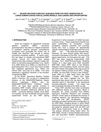
10 member CAM ensemble, with physics diversitya key ingredient in the ensemble. Specifically, 6 ofthe 10 members started with identical initialconditions, but different combinations ofmicrophysicalandboundary-layerparameterizations; the other 4 members usedSREF6-based variations in IC and LBC, but alsodifferent combinations of the same physicalparameterizations. A simple plot of the arealcoverage of precipitation as a function of forecasttime (averaged over all days during SE2007)reveals the strong sensitivity to formulations forboth microphysics and BL processes (Fig. 10).Although there were not enough variations toperform a complete separation of contributionsfrom the different parameterizations, one can gaina qualitative sense of the individual biases bygrouping together all forecasts produced using agiven parameterization and computing thedeviation of each group from the mean. When thisis done, it suggests that the MYJ BL scheme tendsto be wetter than YSU, while Ferrier is the wettestmicrophysical parameterization, followed byWSM6 and Thompson. The sensitivities are quitelarge, but it is unclear at this stage which particularschemes are “best” for a given application.Development and refinement of physicalparameterizations remains one of the greatestFig. 10. Percent coverage of precipitation rate 5 mm h-1as a function of forecast hour for all members of theCAPS ensemble, averaged over all days duringSE2007. Microphysical and planetary-boundary-layerparameterizations for the individual members listed inthe legend can be found in Table 2. Stage IIprecipitation observations are represented by the redcurve.6Short-Range Ensemble Forecasting system fromNCEP (Du et al. 2004)10challenges for the modeling community (e.g.,Mass 2006)4. OPPORTUNITIESAs a new class of NWP models, CAMsprovide both researchers and forecasters withnumerous opportunities.Some of theseopportunities represent “low hanging fruit”, whileothers will require years of development.4.1 The Low Hanging Fruit: PostprocessingOpportunities.By definition, CAM configurations allow awhole new set of phenomena to developcompared to coarser resolution models that relyon parameterized convection.Thus, it isincumbent upon numerical modelers to developpost-processing strategies that extract informationabout these phenomena to use as guidance forforecasters.4.1.1 Identification of a new set of simulatedphenomenaThe mesoscale organizational mode ofconvection is an important concern for severeweather forecasters, such as those at the SPC,because the type of severe convection that occursis strongly linked to mode.For example,tornadoes and large hail are often associated withsupercells, while damaging straight-line winds arethe primary threat from bowing line segments.Thus, efforts to identify and characterizeconvective mode in CAM output are providingimportant contributions to new and uniqueforecaster-guidance products.Simulated reflectivity, computed directly frommodel hydrometeor fields, has proven to be veryuseful for subjective assessments of convectivemode. In particular, simulated reflectivity fieldscan provide important clues about structures andcirculations associated with precipitation features(see Koch et al. 2005) and they are very valuablefor comparison with observed reflectivity patterns(as demonstrated in the previous section).Subjective assessments can become evenmore useful when they are combined withobjective routines that identify and highlightspecific features in CAM output. For example,NSSL scientists and SPC forecasters developedseveral diagnostic routines to identify lower tomiddletroposphericrotatingupdraftsinpreparation for SE2005. One of these routinesspecifically identifies updraft helicity and it has

proven to be a useful proxy for supercells in theCAM output (Kain et al. 2008). This is significantbecause supercellular convection produces adisproportionate share of severe convectiveweather (i.e., tornadoes, damaging winds, and/orlarge hail). Fig. 11a zooms in on a 23 h forecastof simulated reflectivity over northern Kansas andsouthern Nebraska, with purple hatching indicatinghigh UH values. Note that the reflectivity patternof the dominant storm resembles that of aprototypical supercell, and the UH diagnosticprovides additional confidence that this is indeed asupercellular structure, as a UH maximum islocated above the inflow notch where one wouldexpect to find a mesocyclone in a storm with thisconfiguration. Although it is unreasonable toexpect the model to routinely have skillful, timely,and reliable predictions of individual storms likethis, it is worth noting that a storm havingsupercellular characteristics was observed in thissame county within about 2 hours of the predictedabFig. 11. a) Simulated 1 km AGL reflectivity from the WRFNSSL 4 km forecast, with area of UH 25 m2 s-2indicated by purple hatching and b) observed mosaic oflowest-elevation-angle radar reflectivity. The validtime is 2300 UTC for the model forecast and 2054UTC for the observations, 31 May 2007, and theindicated county outlines are in northern Kansas andsouthern Nebraska.11storm (Fig. 11b)As discussed in Kain et al. (2008), the UHdiagnostic has proven to be quite useful forhighlighting areas and conditions that favorsupercell formation. SPC forecasters/scientistshave also developed routines that identify othermanifestations of convective mode, such as quasilinear and bowing reflectivity structures. Explicitforecasts of convective mode have proven to beuseful for SPC forecasters. Ongoing efforts areaimed at determining how such informationcompares to inferences made from environmentalparameters.4.1.2Tracking severe phenomena everytimestep.Traditionally, NWP guidance is presented as aseries of snapshots in time (an exception isaccumulated precipitation). This approach hasbeen adequate for most applications becausecommon features of interest evolve slowlycompared to the time between outputs. In CAMS,output frequency is typically no higher than hourly,partly because higher frequency output couldoverwhelm operational dataflow and processingsystems due to the size of the output files. Yetconvective features of interest can develop, move,and vary in intensity on time scales much shorterthan one hour. Thus, we have modified the WRFcode to track certain fields and features every timestep (24 s) while outputting the average orextreme values of the data at normal outputintervals. This approach allows us to monitorphenomena of interest every time step ing an overflow of data.This concept is currently being used to extractsub-output-time information about convectivestorms in WRF-NSSL forecasts, initially focusingon five different output fields. The first two areupdraft and downdraft velocities below the 400hPa level.These two fields have obviousimplications regarding the intensity of convectiveoverturning. The third field is simulated reflectivitycomputed at the lowest model level. Withoutmuch additional computational effort, other levels(or a composite reflectivity field) could be used aswell. As with updraft and downdraft velocities, thisfield is related to the intensity of convection andmay provide some guidance for forecasting largehail, even though hail is not explicitly representedin the current microphysical scheme (WSM6). Thefourth field is 10-m wind speed, which may behelpful in predicting the magnitude of convectivelygenerated surface wind gusts. The last field is

UH. Each of these fields is tracked every timestep at every grid point and 2-D fields representingthe maximum value over the hour (again, at eachgrid point) are saved along with normal outputfields at the top of the hour.This approach not only provides informationabout between-output-time maximum values, ityields features such as wind swaths and supercelltracks in the model.For example, Fig. 122300highlights the

2.1 WRF-EMC and WRF-NSSL As described in the introduction, hourly output from 0000 UTC initializations of the WRF-EMC and WRF-NSSL configurations are used by SPC forecasters every day. The two forecasts cover nearly the same domain (Fig. 1), but they differ significantly in their physical parameterizations and dynamic core (Table 1.). Both .