WIXLIB

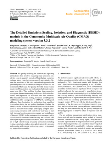
B. N. Murphy et al.: The Detailed Emissions Scaling, Isolation, and Diagnostic (DESID) moduleline (e.g., biogenic and marine vapors, wind-blown dust, seaspray aerosol, lightning-generated nitric oxide) emission input streams (Fig. 1). CMAQ processes each of these types ofstreams differently (US EPA, 2020b): offline gridded emission rates are read in directly as arrays aligned with the modelgrid; offline point emission rates are read in, assigned to theappropriate horizontal row and column, and allocated vertically using source parameters (e.g., stack height, exit velocity, temperature) via buoyancy calculations; and online emissions modules incorporate meteorological (e.g., sunlight, airtemperature, relative humidity, wind speed) and geographical (e.g., land cover classification, leaf area index, oceanfraction) inputs to calculate emission rates. The offline emission inputs, in practice, already include significant chemicalspeciation, whereas the online emission modules must speciate emission rates directly. Despite the differences amongthese three broad categories, DESID structures the flow ofemissions processing within CMAQ so that each emissionstream is retrieved, modified, and diagnosed consistently andthen incorporated independently. Once emissions are calculated they are introduced to the model atmosphere as part ofthe solution for vertical diffusion, which is the first operatorsolved during the model synchronization time step (Byun etal., 1999).Previous versions of CMAQ (5.2.1 and before) and manyother CTMs employ processing approaches that vary amongemissions streams. There are several reasons for these inconsistencies. Models become more complex over time due toincreased computational capabilities and the evolving understanding of air pollution sources over multiple decades. Inaddition, there is a general lack of resources available formodel refactoring and infrastructure development. For example, as Fig. 2 illustrates, CMAQv5.2.1 read emissions of gasphase pollutants from offline gridded emissions, proceededthrough several online and offline point streams, and then finally read all aerosol emissions at the same time. Becausegas and aerosol emissions from the same streams were readand incorporated separately, transparent online scaling wasnot possible. Additionally, CMAQ could read at most oneoffline gridded emission input file and several offline pointinput files. Because of this limitation, sector-specific gridded streams were merged prior to input in CMAQ. Thus, allsector-specific information was lost prior to inclusion in theCMAQ model, and individual sectors required modificationand reprocessing of upstream files.To overcome these and other limitations, DESID makesuse of a series of generalized subroutines developed to handle critical processing steps like emission rate retrieval, errorchecking (e.g., for negative values), size distribution allocation, and unit conversions of all emissions streams (Fig. 3).With this uniform approach in place, model users and developers can be confident that emissions are treated as expectedacross all streams. If sector-specific streams are provided for2-D input (e.g., on-road and non-road vehicles, residentialwood burning, volatile chemical products) rather than ged 2-D input file, DESID may be used to modify thosespecific emission sources. Although this requires more diskspace to store the data needed to drive CMAQ, for many applications the added flexibility justifies the increased storagecost. Several features that accommodate common emissionsprocessing tasks and alleviate workflow bottlenecks for research and regulatory applications build upon this robust system.The rest of this section demonstrates the most useful features that have been incorporated into DESID to date. Webegin with an explanation of the “Emission Control Interface”, a Fortran namelist file that specifies all rules and definitions for DESID behavior. We specifically address how toadd or perturb emissions of chemical species from any emission stream, incorporate spatial dependence, expand scalingto multiple species or streams, ensure mass or mole conservation, and prescribe aerosol size distributions. At this time,DESID does not support rules that vary in time (e.g., application of custom diel temporal profile), but this feature isplanned for a future release. Finally, we introduce the various features available for documenting the data received byCMAQ from each emissions stream and the operations executed by DESID.2.22.2.1Working with DESIDInterfaceThe Emission Control Interface (ECI) provides a flexibleand readable (by the user) platform for directing the behavior of DESID. It is designed to accommodate typicalCMAQ simulation configurations, basic perturbation cases,and highly complex scaling or mapping changes with minimal input lines arranged in a clear and concise layout. Itmanages these tasks while referencing several environmentvariables defined in the CMAQ runscript, including aliasesfor offline emission streams. The publicly available code forCMAQv5.3 and beyond contains default versions of the ECIto support emissions mapping for every supported chemical mechanism including the following: Carbon Bond 6; theSAPRC07 (Statewide Air Pollution Research Center) mechanism, and the RACM2 (Regional Atmospheric ChemistryMechanism). Without the ECI, CMAQ assumes that emissions are zero for all chemical species.The ECI comprises four components to support its breadthof features: Emissions Scaling, Region definitions, Familydefinitions, and Aerosol Size Distribution definitions (Fig. 4and Sect. S1 in the Supplement). The Emissions Scalingcomponent includes all high-level rules to be executed,whereas the remaining three components provide definitionsfor more specific scaling choices. First, we demonstrate common scaling rules possible in the Emissions Scaling component that do not require additional definitions from the support components. The Region, Family, and Aerosol Size Distribution definitions are described subsequently. AdditionalGeosci. Model Dev., 14, 3407–3420, 2021

3410B. N. Murphy et al.: The Detailed Emissions Scaling, Isolation, and Diagnostic (DESID) moduleFigure 1. Example of potential emissions streams and data sources used that inform CMAQ. The offline streams and emission modelsdepicted are not an exhaustive list of all data sources that contribute to a standard CMAQ simulation for the US.Figure 2. Algorithm for emission processing used by CMAQv5.2.1 and previous versions.details and tutorials can be found in the CMAQ user guide(see the “Code and data availability” section for more information).2.2.2Emissions scalingThe Emissions Scaling component is formatted as a tablewith a user-defined number of rows, each corresponding toan individual rule. These rules may be logistically simple(e.g., map the variable named NO from one emissions streamdirectly to the CMAQ species NO) or considerably complex(e.g., scale multiple species by 75 % that have already beenmapped for all emission streams). During the CMAQ initialization process, DESID reads these rules and translates theminto a series of low-level instructions that are stored in severalpersistent arrays. These arrays are then applied uniformly inGeosci. Model Dev., 14, 3407–3420, 2021time to the base emissions after calculation (for online emissions) or interpolation (for offline emissions). Each instruction involves at most one emission stream, one CMAQ variable, and one emission variable. The simplest rules usuallytranslate to one instruction, but the more complex ones (e.g.,affecting multiple streams or multiple CMAQ species) aremade up of several instructions. If no rules are provided toDESID or an ECI is not specified, then CMAQ will introduce no emissions to the model.Each rule is articulated with eight fields (Table 1). Examples 1 and 2 in Table 2 demonstrate rules to map NO and finemode elemental carbon (EC), respectively, for all emissionstreams. In example 2, PEC identifies the particulate elemental carbon from the emissions speciation while AEC identifies the aerosol elemental carbon in the air quality model.In typical cases, the emission variables in these exampleshttps://doi.org/10.5194/gmd-14-3407-2021

B. N. Murphy et al.: The Detailed Emissions Scaling, Isolation, and Diagnostic (DESID) module3411Figure 3. Algorithm for emission stream processing used by DESID. Emission rates are processed for each emission stream independentlybefore DESID proceeds to the next stream.Figure 4. Schematic of Emission Control Interface (ECI) and flow of input options among individual components. Information flow linesare colored based on the component of origin. Text in blue indicates elements that should refer to environment variables set in the CMAQrunscript except in the case where stream labels are populated from the Family component with members that then refer to the runscript. The“Distribution reference” of the Aerosol Size Distribution component refers to entries populated within the CMAQ source code.will be populated by an upstream emission processor during a chemical speciation step that converts emission inventory pollutants to model-relevant species. A broader emission inventory variable like total volatile organic compounds(VOCs) or particulate matter (PM) may be used if it is available on the emission stream. In that case, any scaling ruleswould apply uniformly to all sources that contribute to thatemission stream. For these examples, the add (“a”) operator is used in the “Op” field, indicating that these emissionsshould be added to the system. More complicated scalingrules are possible by exercising options in the available fields.Example 3 shows how to modify the instructions created byExample 1 so that NO emissions are multiplied by 0.8 us-https://doi.org/10.5194/gmd-14-3407-2021ing the multiply “m” operator. Example 4 achieves the sameresult but using the overwrite operator “o”. Because DESIDprocesses rules in the order they are provided in the ECI, ifthe “m” operator were used in Example 4, the scale factor applied to all NO emissions would equal 0.64 (0.8 0.8). The“a” operator may be used for a rule with the same emissionsand CMAQ variables to add or subtract emissions by usingpositive or negative scale factors. For example, if Example 1appeared twice in the ECI, then 200 % of the NO emissionswould be incorporated into the CMAQ simulation.Examples 5 and 6 demonstrate the approach to add multiple emission variables together to contribute to one CMAQvariable. In this case, particulate organic carbon (POC) andGeosci. Model Dev., 14, 3407–3420, 2021

3412B. N. Murphy et al.: The Detailed Emissions Scaling, Isolation, and Diagnostic (DESID) moduleTable 1. Fields required for articulating emission scaling rules in DESID.Field NameDescriptionRegion labelThe region label identifies the region over which the rule is to be applied. The keyword EVERYWHERE appliesthe rule to all grid cells.Stream labelThe stream label identifies the emission streams for which the rule is to be applied. These labels are definedfor offline gridded and point sources in the CMAQ runscript. Online emission streams use keywords including BIOG (biogenic vapors), MGEM (marine gas), LTNG (lightning NO), WBDUST (wind-blown dust), andSEASPRAY (sea spray aerosol). The keyword ALL applies the rule to all streams, including online streams.Emission variableThe emission variable identifies the variable from the emission stream file or online module that emissionsshould be mapped from. The keyword ALL may be used to apply the rule to all previously mapped variables.CMAQ speciesCMAQ species identifies the variable within CMAQ that the rule should be applied to. The keyword ALL maybe used to apply the rule to all previously mapped Species.Phase/ModePhase/Mode is used to distinguish gas or aerosol calculations. If the CMAQ variable is a gas, this field shouldbe set to GAS; if it is an aerosol, this field should indicate the desired aerosol mode (e.g., COARSE, FINE, orother user-defined options) or use the keyword AERO to apply the rule to the entire distribution.Scale factorThe scale factor is a real-valued number applied for scaling calculations.BasisBasis determines whether mass or moles are conserved during conversion from gas to particle emission rates orvice versa. The keyword MASS conserves mass, MOLE conserves moles, and UNIT performs no conversions.OpOp determines the operation for each rule to apply: “a” adds the rule to the existing instruction set and couldalso modify an existing scale factor, “m” finds existing instructions matching this rule’s features (i.e., emissionvariable names, model species, and stream labels) and multiplies their existing scale factors by this rule’s scalefactor, “o” finds existing instructions matching this rule’s features and overwrites their scale factors with thisrule’s scale factor.particulate non-carbon organic matter (PNCOM) are combined to contribute to the emissions of aerosol primary organic matter (APOM). If one wants to scale the CMAQ variable, APOM in this case, it would usually make sense to scalethe rates of both contributing emissions variables, POC andPNCOM. This can be achieved using Example 7, which multiplies the emissions of APOM for both emission variablesby 150 %. Example 8 demonstrates how subtraction may beused to return the emissions of APOM to its original 1 : 1mapping with the emission streams.The examples so far have assumed that the units of theemissions and CMAQ variables are equivalent. However, gasemissions in CMAQ are specified in molar units (mol s 1 ),whereas aerosols are in mass units (g s 1 ) per grid cell. Inorder to map emissions variables to CMAQ species with differing units as in Example 9, the basis field is helpful for prescribing unit conversions. Example 9 has dictated that massbe conserved when scaling additional emissions of APOMfrom gas-phase carbon monoxide (CO) from all streams. Inthis case, DESID will first convert the emission rate of COto mass units using the molecular weight of CO and thenmultiply by the scale factor (2 %). If MOLE were chosen instead, DESID would (in this case) first scale CO emissionsto 2 % (as gas-phase species are typically provided by mole)and then convert to mass units (as aerosol species are trackedin CMAQ in terms of mass) using the molecular weight ofGeosci. Model Dev., 14, 3407–3420, 2021APOM. In examples 1–8 and 10, no unit conversions are performed. To perform mass- and mole-conserving calculations,DESID must know the molecular weight of any emissionvariable to be converted. A table (EMIS SURR TABLE) isprovided within the CMAQ source code (EMIS VARS.F)that stores the molecular weights of all of the known emission variables produced by SMOKE. New emission variablesand corresponding molecular weights should be added to thistable as needed.Finally, another common need for emission sensitivitycases is to target one emission stream for mapping or scaling modification. Example 10 demonstrates a rule for overwriting the scale factor for NO emissions to 200 %, but onlyfor the offline stream labeled ONROAD. Labels for offlinegridded and point streams are set in the CMAQ runscript using environment variables of the GR EMIS LAB xxx andSTK EMIS LAB yyy formats, respectively. The xxx andyyy indices correspond to the environment variables thatstore the file names of each offline stream, GR EMIS xxxand STK EMIS yyy, respectively. Online streams have default stream labels that may be used for scaling rules (see Table 1). An important consideration when designing an emissions input dataset is the level of source detail – DESID canonly modify emissions for a specific source if that source isprovided as its own stream.https://doi.org/10.5194/gmd-14-3407-2021

B. N. Murphy et al.: The Detailed Emissions Scaling, Isolation, and Diagnostic (DESID) moduleAs stated earlier, DESID scaling rules are applied uniformly in time, and there is currently no ability to redistributeemissions in time (e.g., modify the diel profile of a stream orspecies). DESID is unaware of any hourly or daily variabilityin offline emissions, so this feature should be captured using upstream emissions processing tools. By default, DESIDwill generate an error if it finds that the model simulationday does not match the day defined in an offline emissioninput file. It is common for emissions platforms to use representative days for particular offline streams (e.g., weekend–weekday, weekly, monthly, seasonal). In these cases, thedate-matching requirement in DESID may be overriddenby setting the environment variables of the GR EM SYMDATE xxx and STK EM SYM DATE yyy formats to true.2.2.3Region definitionsThe Region definitions component of the ECI maps labels forgridded spatial arrays to the geographic input files and variables containing data for those arrays. Each entry or row inthis component contains three fields (Table 3), which identify the input file and target variable to be associated with aspecific region. The data for each region are expected to alignwith the simulation domain resolution and projection and include real numbers between 0 and 1.0, quantifying the fraction of emissions in each model grid cell that is associatedwith the region. Common examples of regions used for scaling include political areas like countries, states, or counties,or geographical features like oceans, lakes, or forests. Datafiles containing variables describing political boundaries areavailable for a typical 12 km continental US domain from theCommunity Modeling and Analysis System Data Warehouse(US EPA, 2019b). Tutorials demonstrating a process for creating custom region variables for any grid using open-sourcetools will be available in future CMAQ repositories. As described in Table 3, if all the variables in the input file aredesired (e.g., all of the lower 48 US states), the ALL keyword may be used for the region label and target variable toinstruct DESID to make all of the variables on the input fileavailable as regions, reducing the number of input lines from48 to 1. There is no limit to the number of input files that maybe referenced and read to define regions in DESID.Table 4 demonstrates three examples defining regions ofincreasing size – a US city (Chicago), a US state (Illinois),and a broader US geographical area (the Ohio Valley), are alldefined. A hypothetical use case for prescribing NO2 emissions using these regions is shown in Table 5. Example 11maps the NO2 emissions variable to the CMAQ NO2 variable for the entire domain. Example 12 articulates a sensitivity whereby emissions in the Ohio Valley are cut by 30 %.Examples 13 and 14 refine this perturbation with further spatial detail, overwriting the 30 % cut with a 10 % increase andan 80 % decrease in emissions for the state of Illinois andthe Chicago area, respectively. Thus, the Region definitionfeature facilitates implementation of highly refined 413dependent emissions sensitivity experiments within CMAQ.However, these modifications are currently only possible atthe resolution of the simulation grid. The ECI for enforcingExample 13 and the resulting fields of emission and NO2concentration changes are given in the Supplement (Sect. S2and Fig. S1).Although DESID’s region-based scaling capability is useful for many applications, it can introduce potentially important uncertainties when the scale of the model grid is insufficient for capturing the distribution of pollutants betweentwo neighboring boundaries. For example, consider a regionmask specifying the domain of Illinois including real fractions that are area weighted. If a hypothetical border grid cellcontains far more Illinois emissions from some sector thanthe area-weighted fraction would indica

model refactoring and infrastructure development. For exam-ple, as Fig. 2 illustrates, CMAQv5.2.1 read emissions of gas-phase pollutants from offline gridded emissions, proceeded through several online and offline point streams, and then fi-nally read all aerosol emissions at the same time. Because