WIXLIB

Mahalanobis distance learningMore on the Mahalanobis distanceRecapThe Mahalanobis (pseudo) distance is defined as follows:qdM (x, x0 ) (x x0 )T M(x x0 ),where M Rd d is a symmetric PSD matrix.InterpretationEquivalent to a Euclidean distance after a linear projection L:qqdM (x, x0 ) (x x0 )T M(x x0 ) (x x0 )T LT L(x x0 )q (Lx Lx0 )T (Lx Lx0 ).If M has rank k, L Rk d (dimensionality reduction).RemarkFor convenience, often use the squared distance (linear in M).29 / 122

Mahalanobis distance learningMMC [Xing et al., 2002]FormulationmaxM Rd ds.t.XdM (xi , xj )(xi ,xj ) DX2dM(xi , xj ) 1,(xi ,xj ) SM 0.RemarksProposed for clustering with side information.The problem is convex in M and always feasible (with M 0).Solved with a projected gradient descent algorithm.For large d, the bottleneck is the projection on the set M 0:requires eigenvalue decomposition which scales in O(d 3 ).Only look at sum of distances.30 / 122

Mahalanobis distance learningMMC [Xing et al., 2002]Projected data505000zzOriginal data 50 5050y50500 50yxionosphere (N 351, C 2, d 34)10.80.80.60.60.40.40.20.2few constraintsmore constraints 500 50xprotein (N 116, C 6, d 20)105000 500few constraintsmore constraintsleft to right: K-Means, K-Means MMC-Diag, K-Means MMC-Full, Constrained K-Means31 / 122

Mahalanobis distance learningS&J [Schultz and Joachims, 2003]FormulationminMkMk2F22s.t. dM(xi , xk ) dM(xi , xj ) 1 (xi , xj , xk ) RM 0,RemarksRegularization on M (keeps the metric “simple”, avoid overfitting).One large-margin constraint per triplet.32 / 122

Mahalanobis distance learningS&J [Schultz and Joachims, 2003]Formulation with soft constraintsminM,ξ 0kMk2F CPi,j,k ξijk22s.t. dM(xi , xk ) dM(xi , xj ) 1 ξijk (xi , xj , xk ) RM 0,RemarksRegularization on M (keeps the metric “simple”, avoid overfitting).One large-margin constraint per triplet that may be violated.Advantages:more flexible constraints.32 / 122

Mahalanobis distance learningS&J [Schultz and Joachims, 2003]Formulation with soft constraints and PSD enforcement by designminW,ξ 0kMk2F CPi,j,k ξijk22s.t. dM(xi , xk ) dM(xi , xj ) 1 ξijk (xi , xj , xk ) RX MX X0,X where M AT WA, where A is fixed and known and W diagonal.RemarksRegularization on M (keeps the metric “simple”, avoid overfitting).One large-margin constraint per triplet that may be violated.Advantages:more flexible constraints.no PSD constraint to deal with.Drawbacks:how to choose appropriate A?only learns a weighting of the attributes defined by A.32 / 122

Mahalanobis distance learningNCA [Goldberger et al., 2004]Main ideaOptimize leave-one-out error of a stochastic nearest neighbor classifier inthe projection space induced by dM . Use M LT L and define theprobability of xj being the neighbor of xi aspij Pexp( kLxi Lxj k22 ), pii 0.2l6 i exp( kLxi Lxl k2 )FormulationmaxLwhere pi Pj:yj yiPipi ,pij is the probability that xi is correctly classified.RemarksFully supervised, tailored to 1NN classifier.Can pick L rectangular for dimensionality reduction.Nonconvex (thus subject to local optima).33 / 122

Mahalanobis distance learningNCA [Goldberger et al., 2004]34 / 122

Mahalanobis distance learningLMNN [Weinberger et al., 2005]Main IdeaDefine constraints tailored to k-NN in a local way: the k nearest neighborsshould be of same class (“target neighbors”), while examples of differentclasses should be kept away (“impostors”):S {(xi , xj ) : yi yj and xj belongs to the k-neighborhood of xi },R {(xi , xj , xk ) : (xi , xj ) S, yi 6 yk }.35 / 122

Mahalanobis distance learningLMNN [Weinberger et al., 2005]FormulationminM Sd ,ξ 0(1 µ)X2dM(xi , xj ) µ(xi ,xj ) SXξijki,j,k22s.t. dM(xi , xk ) dM(xi , xj ) 1 ξijk (xi , xj , xk ) R,where µ [0, 1] is a trade-off parameter.RemarksMinimizing the distances between target neighbors as a regularizer.Advantages:More flexible constraints (but require full supervision).Convex, with a solver based on working set and subgradient descent.Can deal with millions of constraints and very popular in practice.Drawbacks:Subject to overfitting in high dimension.Sensitive to Euclidean distance performance.36 / 122

Mahalanobis distance learningITML [Davis et al., 2007]Main ideaUse a regularizer that automatically enforces PSD, the LogDet divergence: 1Dld (M, M0 ) tr(MM 10 ) log det(MM0 ) d XX λiλiT2log (vi ui ) d,θjθii,jiwhere M VΛVT and M0 UΘUT is some PSD matrix (typically I orΣ 1 ). Properties:Convex (because determinant of PSD matrix is log-concave).Finite if and only if range(M) range(M0 ).Implicitly makes M PSD and same rank as M0 .Information-theoretic interpretation: minimize KL divergence betweentwo Gaussians parameterized by M and M0 .37 / 122

Mahalanobis distance learningITML [Davis et al., 2007]FormulationminM Sd ,ξ 0Dld (M, M0 ) λXξiji,j2s.t. dM(xi , xj ) u ξij2dM(xi , xj ) v ξij (xi , xj ) S (xi , xj ) D,where u, v , λ 0 are threshold and trade-off parameters.RemarksSoft must-link / cannot-link constraints.Simple algorithm based on Bregman projections. Each iteration isquadratic in d instead of cubic with projections on PSD cone.Drawback: the choice of M0 can have an important influence on thequality of the learned metric.38 / 122

Mahalanobis distance learningOnline learningLarge-scale metric learningConsider the situation where the number of training constraints isvery large, say 106 (this can happen even with a moderate numberof training examples, e.g. in LMNN).Previous algorithms become huge, possibly intractable optimizationproblems (gradient computation and/or projections become veryexpensive).One solution: online learningIn online learning, the algorithm receives training instances one at atime and updates the current hypothesis at each step.Performance typically inferior to that of batch algorithms, but allowsto tackle large-scale problems.39 / 122

Mahalanobis distance learningOnline learningSetup, notations, definitionsStart with a hypothesis h1 .At each step t 1, . . . , T , the learner receives a training examplezt (xt , yt ) and suffers a loss (ht , zt ). Depending on the loss, itgenerates a new hypothesis ht 1 .The goal is to find a low-regret hypothesis (how much worse we docompared to the best hypothesis in hindsight):R TXt 1 (ht , zt ) TX (h , zt ),t 1where h is the best batch hypothesis on the T examples.Ideally, have a regret bound of the form R O(T ).40 / 122

Mahalanobis distance learningLEGO [Jain et al., 2008]FormulationAt each step, receive (xt , x0t , yt ) where yt is the target distance between xtand x0t , and update as follows:Mt 1 arg min Dld (M, Mt ) λ (M, xt , x0t , yt ),M 0where is a loss function (square loss, hinge loss.).RemarksIt turns out that the above update has a closed-form solution whichmaintains M 0 automatically.Can derive a regret bound.41 / 122

Linear similarity learningMotivationDrawbacks of Mahalanobis distance learningMaintaining M 0 is often costly, especially in high dimensions. Ifthe decomposition M LT L is used, formulations become nonconvex.Objects must have same dimension.Distance properties can be useful (e.g., for fast neighbor search), butrestrictive. Evidence that our notion of (visual) similarity violates thetriangle inequality (example below).42 / 122

Linear similarity learningOASIS [Chechik et al., 2009]RecapThe bilinear similarity is defined as follows:KM (x, x0 ) xT Mx0 ,where M Rd d is not required to be PSD nor symmetric. In general, itsatisfies none of the distance properties.FormulationAt each step, receive triplet (xi , xj , xk ) R and update as follows:Mt arg minM,ξ 01kM Mt 1 k2F C ξ2s.t. 1 KM (xi , xj ) KM (xi , xk ) ξ.43 / 122

Linear similarity learningOASIS [Chechik et al., 2009]FormulationAt each step, receive triplet (xi , xj , xk ) R and update as follows:Mt arg minM,ξ 01kM Mt 1 k2F C ξ2s.t. 1 KM (xi , xj ) KM (xi , xk ) ξ.RemarksPassive-aggressive algorithm: no update if the triplet satisfies themargin. Otherwise, simple closed-form update.Scale to very large datasets with good generalization performance.Evaluated on 2.3M training instances (image retrieval task).Limitation: restricted to Frobenius norm (no fancy regularization).44 / 122

Linear similarity learningOASIS [Chechik et al., 2009]45 / 122

Linear similarity learningSLLC [Bellet et al., 2012b]Main ideaSimilarity learning to improve linear classification (instead of k-NN).Based on the theory of learning with ( , γ, τ )-good similarity functions[Balcan et al., 2008]. Basic idea: use similarity as features (similarity map).K(x,E)If the similarity satisfies some property, then there exists a sparse linearclassifier with small error in that space (more on this later).EFHGCDABK(x,A)K(x,B)46 / 122

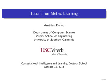
Linear similarity learningSLLC [Bellet et al., 2012b]FormulationminM Rd d1nnXi 1 1 yi 1γ R Xxj Ryj KM (xi , xj ) βkMk2F , where R is a set of reference points randomly selected from the trainingsample, γ is the margin parameter, [·] is the hinge loss and β theregularization parameter.RemarksBasically learn KM such that training examples are more similar onaverage to reference points of same class than to those of oppositeclass by a margin γ. Thus, more flexible constraints that are sufficientfor linear classification.Leads to very sparse classifiers with error bounds (more on this later).Drawback: multi-class setting requires several classifiers.47 / 122

Linear similarity learningSLLC [Bellet et al., 2012b] 5KI (0.50196)0.380.260.1402 0.10 0.2 2 0.3 4 0.4 0.4 0.200.20.4SLLC (1)x 10 6 0.01 0.005LMNN (0.85804)00.0050.010.015ITML (0.50002)300.3200.20.11000 0.1 10 0.2 20 30 30 0.3 20 1001020 0.4 0.4 0.200.20.448 / 122

Linear similarity learningSLLC [Bellet et al., 2012b] 5KI (0.69754)104SLLC (0.93035)x 10352010 5 1 10 15 20 2 1001020 3 1 0.500.51 4x 10LMNN (0.80975)ITML (0.97105)50010.80.60.400.20 0.2 500 1000 50005001000 0.4 20 100102049 / 122

Linear metric learningSummary and limitationSummaryWell-studied framework, often with convex formulations.Can learn online (or using stochastic gradient) to scale to largedatasets.Mahalanobis if distance properties are needed, otherwise moreflexibility with a similarity function.LimitationA linear metric is often unable to accurately capture the complexity of thetask (multimodal data, nonlinear class boundaries).50 / 122

Outline1PreliminariesMetrics, basic notions of convex optimization2Metric Learning in a NutshellBasic formulation, type of constraints, key properties3Linear Metric LearningMahalanobis distance learning, similarity learning4Nonlinear Metric LearningKernelization of linear methods, nonlinear and local metric learning5Metric Learning for Other SettingsMulti-task, ranking, histogram data, semi-supervised, domain adaptation6Metric Learning for Structured DataString and tree edit distance learning7Deriving Generalization GuaranteesBasic notions of statistical learning theory, the specifics of metric learning8Summary and Outlook51 / 122

Nonlinear metric learningThe big pictureThree approaches1Kernelization of linear methods.2Learning a nonlinear metric.3Learning several local linear metrics.52 / 122

Nonlinear metric learningKernelization of linear methodsDefinition (Kernel function)A symmetric similarity function K is a kernel if there exists a (possiblyimplicit) mapping function φ : X H from the instance space X to aHilbert space H such that K can be written as an inner product in H:K (x, x 0 ) φ(x), φ(x 0 ) .Equivalently, K is a kernel if it is positive semi-definite (PSD), i.e.,n XnXci cj K (xi , xj ) 0i 1 j 1for all finite sequences of x1 , . . . , xn X and c1 , . . . , cn R.53 / 122

Nonlinear metric learningKernelization of linear methodsKernel trickLet K (x, x 0 ) hφ(x), φ(x 0 )i a kernel. We have training data {xi }ni 1 anddefwe use φi φ(xi ). We want to compute a (squared) Mahalanobisdistance in kernel space:2dM(φi , φj ) (φi φj )T M(φi φj ) (φi φj )T LT L(φi φj ).Let Φ [φ1 , . . . , φn ] and use the parameterization LT ΦUT . Now:2dM(φi , φj ) (ki kj )T M(ki kj ),where ki ΦT φi [K (x1 , xi ), . . . , K (xn , xi )]T and M is n n.54 / 122

Nonlinear metric learningKernelization of linear methodsNow, why is this interesting?Similar trick as in kernel SVM: take K to be some nonlinear kernel.Say, the RBF kernel (inducing an infinite dimensional space): kx x0 k220.Krbf (x, x ) exp 2σ 2We get a distance computed after a nonlinear, high-dimensionalprojection of the data, but distance computations are doneinexpensively through the kernel.To learn our distance, need to estimate n2 parameters: independentof original and projection space dimensions!Justified theoretically through a representer theorem[Chatpatanasiri et al., 2010].55 / 122

Nonlinear metric learningKernelization of linear methodsLimitationsSome algorithms have been shown to be kernelizable, but in generalthis is not trivial: a new formulation of the problem has to be derived,where interface to the data is limited to inner products, andsometimes a different implementation is necessary.When the number of training examples n is large, learning n2parameters may be intractable.A solution: KPCA trickUse KPCA (PCA in kernel space) to get a nonlinear butlow-dimensional projection of the data.Then use unchanged algorithm!Again, theoretically justified [Chatpatanasiri et al., 2010].56 / 122

Nonlinear metric learningLearning a nonlinear metric: GB-LMNN [Kedem et al., 2012]Main ideaLearn a nonlinear mapping φ to optimize the Euclidean distancedφ (x, x0 ) kφ(x) φ(x0 )k2 in the transformed space.Same objective as LMNN.PThey use φ φ0 α Tt 1 ht , where φ0 is the mapping learned bylinear LMNN, and h1 , . . . , hT are gradient boosted regression trees oflimited depth p.At iteration t, the tree that best approximate the negative gradient gt of the objective with respect to the current transformation φt 1 :nX(gt (xi ) h(xi ))2 .ht (·) arg minhi 1Intuitively, each tree divides the space into 2p regions, and instancesfalling in the same region are translated by the same vector (thusexamples in different regions are translated in different directions).57 / 122

Nonlinear metric learningLearning a nonlinear metric: GB-LMNN [Kedem et al., 2012]RemarksDimensionality reduction can be achieved by learning trees withlow-dimensional output.The objective function is nonconvex, so bad local minima are anissue, although this is attenuated by initializing with linear LMNN.In practice, GB-LMNN performs well and seems quite robust tooverfitting.Drawback: distance evaluation may become expensive when a largenumber of trees is needed.58 / 122

Nonlinear metric learningLocal metric learningMotivationSimple linear metrics perform well locally.Since everything is linear, can keep formulation convex.PitfallsHow to split the space?How to avoid a blow-up in number of parameters to learn, and avoidoverfitting?How to make local metrics comparable?How to generalize local metrics to new regions?How to obtain a proper global metric?.59 / 122

Nonlinear metric learningLocal metric learning: MM-LMNN [Weinberger and Saul, 2009]Main ideaExtension of LMNN where data is first divided into C clusters and ametric is learned for each cluster.Learn the metrics in a coupled fashion, where the distance to a targetneighbor or an impostor x is measured under the local metricassociated with the cluster to which x belongs.Formulation (one metric per class)minM1 ,.,MC Sd ,ξ 0(1 µ)X2(xi , xj )dMyj µξijki,j,k(xi ,xj ) S22s.t. dM(xi , xk ) dM(xi , xj ) 1 ξijkyykXj (xi , xj , xk ) R.60 / 122

Nonlinear metric learningLocal metric learning: MM-LMNN [Weinberger and Saul, 2009]Formulation (one metric per class)minM1 ,.,MC Sd ,ξ 0(1 µ)X2dM(xi , xj )yj µX22s.t. dM(xi , xk ) dM(xi , xj ) 1 ξijkyykξijki,j,k(xi ,xj ) Sj (xi , xj , xk ) R.RemarksAdvantages:The problem remains convex.Can lead to significant improvement over LMNN.Drawbacks:Subject to important overfitting.Computationally expensive as the number of metrics grows.Change in metric between two neighboring regions can be very sharp.61 / 122

Nonlinear metric learningLocal metric learning: MM-LMNN [Weinberger and Saul, 2009]62 / 122

Nonlinear metric learningLocal metric learning: PLML [Wang et al., 2012]Main idea2 for each training instance x as a weightedLearn a metric dMiicombination of metrics defined at anchor points u1 , . . . , umthroughout the space.First, learn the weights based on manifold (smoothness) assumption.Then, learn the anchor metrics.Weight learningmin kX WUk2F λ1 tr(WG) λ2 tr(WT LW)Ws.t. Wibj 0, i, bjmXWibj 1, i,j 1where G holds distances between each training point and each anchorpoint, and L is the Laplacian matrix constructed on the training instances.63 / 122

Nonlinear metric learningLocal metric learning: PLML [Wang et al., 2012]Anchor metric learningSimilar to (MM)-LMNN.RemarksAdvantages:Both subproblems are convex.A specific metric for each training point, while only learning a smallnumber of anchor metrics.Smoothly varying metrics reduce overfitting.Drawbacks:Learning anchor metrics can still be expensive.No discriminative information when learning the weights.No principled way to get metric for a test point (in practice, useweights of nearest neighbor).Relies a lot on Euc

2 Metric Learning in a Nutshell Basic formulation, type of constraints, key properties 3 Linear Metric Learning Mahalanobis distance learning, similarity learning 4 Nonlinear Metric Learning Kernelization of linear methods, nonlinear and local metric learning 5 Metric Learning for Other Settings