Transcription
Shiken: JALT Testing & Evaluation SIG Newsletter. 12 (2) April 2008 (p. 38 - 43)Statistics CornerQuestions and answers about language testing statistics:Effect size and eta squaredJames Dean Brown (University of Hawai‘i at Manoa)Question: In Chapter 6 of the 2008 book on heritage language learning that you coedited with Kimi-Kondo Brown, a study comparing how three different groups ofinformants use intersentential referencing is outlined. On page 147 of that book, aMANOVA with a partial eta2 of .29 is outlined. There are several questions about thisstatistic. What does a “partial eta” measure? Are there other forms of eta that readersshould know about? And how should one interpret a partial eta2 value of .29?Answer: I will answer your question about partial eta2 in two parts. I will start bydefining and explaining eta2. Then I will circle back and do the same for partial eta2.Eta2Eta2 can be defined as the proportion of variance associated with or accounted forby each of the main effects, interactions, and error in an ANOVA study (seeTabachnick & Fidell, 2001, pp. 54-55, and Thompson, 2006, pp. 317-319).Formulaically, eta2, or η 2 , is defined as follows:SSη 2 effectSStotalWhere:SSeffect the sums of squares for whatever effect is of interestSStotal the total sums of squares for all effects, interactions, and errors in the ANOVAEta2 is most often reported for straightforward ANOVA designs that (a) are balanced(i.e., have equal cell sizes) and (b) have independent cells (i.e., different people appearin each cell). For example, in Brown (2007), I used an example ANOVA todemonstrate how to calculate power with SPSS. That was a 2 x 2 two-way ANOVAwith anxiety and tension as the independent variables and trial 3 as the dependentvariable (using the Anxiety 2.sav example file that comes with recent versions of theSPSS software). There were three people in each cell and the cells were independent.Notice in Table 1 that the p values (0.90, 0.55, & 0.10) indicate that there were nosignificant effects (i.e., no p values below .05) for Anxiety, Tension, or their interaction.Note also that there was not sufficient power to detect such effects (i.e., the powerstatistics of 0.05, 0.09, & 0.37 were not above .80 in any case). All of this led me toconclude that “the study lacked sufficient power to detect any significant effects even ifthey exist in reality”, which is reasonable given the very small sample size of 12.Table 1 Results of the Analysis Shown in Figure 3 of the Anxiety 2.sav used with SPSSSourceSSdfMSFpeta2PowerAnxiety0.0810.08 0.02 0.90 0.00120.05Tension2.0812.08 0.38 0.55 0.03240.09Anxiety x Tension 18.751 18.75 3.46 0.10 0.29190.37Error43.3385.420.6745Total64.24 12
39Table 2 Descriptive Statistics for the Anxiety 2.sav Example Used with SPSS *Anxiety TensionMSD N118.67 3.06 327.00 2.65 3216.00 2.00 329.33 1.16 3*Dependent Variable: Trial 3Nonetheless, even a cursory look at the means shown in Table 2 indicates that fairlylarge differences exist between means and something noteworthy is going on, so abetter designed replication study with a larger sample size might be justified. Eta2 canhelp in interpreting the results by indicating the relative degree to which the variancethat was found in the ANOVA was associated with each of the main effects (Anxietyand Tension) and their interaction.Eta2 values are easy to calculate. Simply add up all the sums of squares (SS), thetotal of which is 64.24 in the example; then, divide the SS for each of the main effects,the interaction, and the error term by that total. The results will be as follows:SS Anxiety0.08 0.00124533 0.0012SSTotal64.24SS2.082ηTension Tension 0.03237858 0.0324SSTotal64.24SS AxT 18.752η AxT 0.291874221 0.2919SSTotal 64.24SS43.332η Error Error 0.674501867 0.6745SSTotal 64.242η Anxiety Interpretation of these values is easiest if the decimal point is moved two places tothe right in each case, the result of which can be interpreted as percentages of varianceassociated with each of the main effects, the interaction, and error.Starting with Anxiety, the value of 0.0012 indicates that a mere 0.12% of thevariance is accounted for by Anxiety, whereas Tension accounts for 3.24%, theAnxiety x Tension (A x T) interaction accounts for a much larger 29.19%, and awhopping 67.45% is accounted for by Error. Now let’s consider the A x T interactionand Error separately in more detail.The 29.19% accounted for by the A x T interaction should lead the researcher tounderstand that this interaction effect is much more important than either of theindividual main effects for Anxiety or Tension, a fact that, even though there are nosignificant effects, may help in designing future studies and understanding why thepresent one did not detect significant differences. Such an important interaction effectshould lead the researcher to want to plot out that relationship as shown in Figure 1,where we see that the Tension groups 1 (dotted line) and 2 (plain black line) do indeedhave different means but in opposite relationships for Anxiety 1 and 2. That is, theTension 1 group is higher than the Tension 2 group when Anxiety is 1, but the Tension1 group is lower than the Tension 2 group when Anxiety is 2.39
40Thus there is a strong pattern but it is not consistent across Anxiety 1 and 2conditions (if it were consistent, the lines would be parallel). Thus, even with a nonsignificant interaction (where p .10), the eta2 value of .2919 drew our attention to animportant interaction effect that is revealing in itself, and which may help tounderstand why there were no significant main effects for Tension or Anxiety (i.e.,because the interaction cancels out any such differences).Figure 1. Interaction of Anxiety with Tension using the Anxiety 2.sav exampleThe whopping 67.45% accounted for by Error in the Table 1 indicates that morethan two-thirds of the variance was not accounted for at all in this design. This errorvariance may be due to unreliable variance in the study due to poor design, othersystematic variables that might be of interest (if they were operationalized and includedin the study), and so forth. All in all, eta2 values indicate not only that the interactioneffect and error are causing almost 97% of the variance in the study (67.45 29.19 96.64), but also ways to redesign the study so it will be more powerful and meaningful.One problem with eta2 is that the magnitude2“One problem with eta is that theof eta2 for each particular effect depends to somemagnitude of eta2 for each particulardegree on the significance and number of othereffect depends to some degree on theeffects in the design (Tabachnick & Fidell, 2001,significance and number of otherp. 54). One statistic that minimizes the effects ofeffects in the design . . .”this issue is called partial eta2.Partial Eta2Partial eta2 can be defined as the ratio of variance accounted for by an effect andthat effect plus its associated error variance within an ANOVA study. Formulaically,40
412partial eta2, or η partial, is defined as follows:2η partial SSeffectSSeffect SSerrorWhere:SSeffect the sums of squares for whatever effect is of interestSSerror the sums of squares for whatever error term is associated with that effectIn applied linguistics studies, partial eta2 is most often reported for ANOVA designsthat have non-independent cells (i.e., the same people appear in more than one cell).For example, in Brown, Hilgers, and Marsella (1991), students wrote compositions ontwo different types of topics (a narrative topic and an analytic topic) which wereorganized into ten prompt sets. The people who wrote on each of the ten prompt setswere different from each other (so this is also known as a between subjects effect). Incontrast, every student wrote on each of the two topic types, so these were treated asrepeated measures (also known as a within subjects effect). The cell sizes withinsubjects were exactly the same (which makes sense because they were the samepeople), whereas the cell sizes between subjects were different to small degrees. Theoriginal results of this 10 x 2 two-way repeated-measures ANOVA for prompt sets andtopic types are shown in Table 3.Table 3 Two-Way Repeated-Measures ANOVA for 1989 Prompt Sets and Topic Types(As presented in Brown et al, 1991)SourceBetween SubjectsPrompt 030.00Within SubjectsTopic TypePrompt Set by Topic 50.1948.6110.660.00Table 4 Two-Way Repeated-Measures ANOVA for 1989 Prompt Sets and Topic Types(Adapted from Brown et al, 1991 with Partial Eta2 Added)SourceSSdfMSFpPartialeta2Between SubjectsPrompt Set (PS)158.3729 17.597 9.703 0.00 0.0490ErrorBS3068.553 16921.814Within SubjectsTopic Type (TT)Prompt Set by Topic 7750.1948.6110.660.000.00010.0438From my present perspective (17 years later), the 1991Brown et al. study wouldhave been strengthened by relabeling the effects and adding partial eta2 values to thetwo-way repeated-measures ANOVA table as shown in Table 4. These partial eta241
42values are easy to calculate. Simply divide the SS for each effect by the SS of thateffect plus the SS for the error associated with that effect. The results will be as follows:SS PS158.3722Partial η PS 0.049078302 0.0490SS PS SS ErrorBS 158.372 3068.5532Partial ηTT SSTT2Partial η PSxTT SSTT0.344 0.000114518 0.0001 SS ErrorWS 0.344 3003.548SS PSxTT137.572 0.043797116 0.0438SS PSxTT SS ErrorWS 137.572 3003.548The interpretation of these partial eta2 values is similar to what we did above for eta2in that we need to move the decimal point two places to the right in each case, andinterpret the results as percentages of variance. However, this time the results indicatethe percentage of variance in each of the effects (or interaction) and its associated errorthat is accounted for by that effect (or interaction). Starting with Prompt Sets, the valueof 0.0490 indicates that 4.90% of the between subjects variance is accounted for byPrompt Sets, whereas Topic Types accounts for nearly none of the TT plus ErrorBSvariance (0.01%), though the Prompt Sets by Topic Types interaction (PSxTT) accountsfor a somewhat larger 4.38% of the PSxTT plus ErrorBS variance.ConclusionIn direct answer to your question, Kondo-Brown and Fukuda (2008) correctly choseto use partial eta2 because their design was a MANOVA, which by definition involvesnon-independent or repeated measures. When they reported that partial eta2 was .29,that meant that the effect for group differences in their MANOVA accounted for 29% ofthe group-differences plus associated error variance as explained above. Thispercentage was sufficient to lead them to do univariate follow-up ANOVAs that helpedthem to further isolate exactly where the significant and interesting means differenceswere to be found.In recent columns, I have covered a number of issues related to the ANOVA sorts ofstudies including: sampling and generalizability, sampling errors, sample size andpower, and effect size and eta squared. All of these are ways to expand your thinkingabout ANOVA—ways that are often ignored in applied linguistics. They have longbeen important to understanding ANOVA results in psychology, education, and otherfields, and we ignore them to our detriment. To paraphrase something one of my statsteachers said back in the late 1970s: Reporting the traditional ANOVA source table(with SS, df, MS, F, and p) and discussing the associated significance levels isn’t theend of the study; it’s just the beginning because we“Reporting the traditional ANOVAcan learn much more by carefully plotting andsource table (with SS, df, MS, F, andconsidering the interaction effects and doing followp) and discussing the associatedup analyses like planned or post-hoc comparisons,significance levels isn’t the end ofpower and effect size analyses, and so forth. Ithe study; it’s just the beginning . . .”hope I have delivered that message loud and clear.References42
43Brown, J. D. (2007). Statistics Corner. Questions and answers about language testing statistics: Samplesize and power. Shiken: JALT Testing & Evaluation SIG Newsletter, 11(1), 31-35. Also retrieved from theWorld Wide Web at http://jalt.org/test/bro 25.htmBrown, J. D., Hilgers, T., & Marsella, J. (1991). Essay prompts and topics: Minimizing the effect ofdifferences. Written Communication, 8(4), 532-555.Kondo-Brown, K. (2005). Differences in language skills: Heritage language learner subgroups and foreignlanguage learners. The Modern Language Journal, 89(4), 563–581.Kondo-Brown, K., & Brown, J. D. (Eds.) (2008). Teaching Chinese, Japanese, and Korean heritagelanguage students. New York: Lawrence Erlbaum Associates.Kondo-Brown, K., & Fukuda, C. (2008). A separate-track for advanced heritage language students?:Japanese intersentential referencing. In K. Kondo-Brown & J. D. Brown (Eds.), Teaching Chinese,Japanese, and Korean heritage language students. New York: Lawrence Erlbaum Associates.Tabachnick, B. G., & Fidell, L. S. (2001). Using Multivariate Statistics (5th ed.). Upper Saddle River, NJ:Pearson Allyn & Bacon.Thompson, B. (2006). Foundations of behavioral statistics: An insight-based approach. New York:Guilford.HTML: http://jalt.org/test/bro 28.htm / PDF: http://jalt.org/test/PDF/Brown28.pdfCopyright 2008 by James Dean Brown & the Japan Association for Language Teaching43
Effect size and eta squared James Dean Brown (University of Hawai‘i at Manoa) Question: In Chapter 6 of the 2008 book on heritage language learning that you co-edited with Kimi-Kondo Brown, a study comparing how three different groups of informants use intersentential referencing is outlined. On page 147 of that book, aFile Size: 376KBPage Count: 6