WIXLIB

thm argument. Since KDT is open-source (available at http://kdt.sourceforge.net), algorithm researchers can look at existing methods to understandimplementation details, to tweak algorithms for theirspecific needs, or to guide the development of new sDiGraphbfsTree,neighbor degree,subgraph load,UFget ,- ‐,sum,scale generators HyGraphtoDiGraph load,Ufget bfsTree degree MatSpMV SpGEMM load,save,eye reduce,scale EWiseApply,[] Vecmax,norm,sort abs,any,ceil range,ones EWiseApply,[] gmethods(SpMV,SpGEMM)Sparse- uce)Figure 4: The architecture of Knowledge DiscoveryToolbox. The top-layer methods are primarily used bydomain experts, and include centrality and clusterfor semantic graphs. The middle-layer methods are primarily used by graph-algorithm developers to implement the top-layer methods. KDT is layered on topof Combinatorial BLAS.tually spectral and k-means algorithms for clustering).Good characterizations of each algorithm’s fitness forvarious types of very large data are rare and so mosttarget users will not know in advance which algorithmswill work well for their data. We expect the set of highlevel methods to evolve over time.The high-level methods are supported by a smallnumber of carefully chosen building blocks. KDT istargeted to analyze large graphs for which parallelexecution in distributed memory is vital, and so itsprimitives are tailored to work on entire collections ofvertices and edges. As the middle layer in Figure 4illustrates, these include directed graphs (DiGraph),hypergraphs (HyGraph), and matrices and vectors (Mat,Vec). The building blocks support lower-level graph andsparse matrix methods (for example, degree, bfsTree,and SpGEMM). This is the level at which the graphalgorithm developer or researcher programs KDT.Our current computational engine is CombinatorialBLAS [8] (shortened to CombBLAS), which gives excellent and highly scalable performance on distributedmemory HPC clusters. It forms the bottom layer of oursoftware stack.Knowledge discovery is a new and rapidly changing field, and so KDT’s architecture fosters extensibility. For example, a new clustering algorithm caneasily be added to the cluster routine, reusing mostof the existing interface. This makes it easy for theuser to adopt a new algorithm merely by changing the3 Related WorkKDT combines a high-level language environment, tomake both domain users and algorithm developers moreproductive, with a high-performance computational engine to allow scaling to massive graphs. Several otherresearch systems provide some of these features, thoughwe believe that KDT is the first to integrate them all.Titan [35] is a component-based pipeline architecture for ingestion, processing, and visualization of informatics data that can be coupled to various highperformance computing platforms. Pegasus [19] is agraph-analysis package that uses MapReduce [11] ina distributed-computing setting. Pegasus uses a generalized sparse matrix-vector multiplication primitivecalled GIM-V, much like KDT’s SpMV, to express vertexcentered computations that combine data from neighboring edges and vertices. This style of programming is called “think like a vertex” in Pregel [27], adistributed-computing graph API. In traditional scientific computing terminology, these are all BLAS-2 leveloperations; neither Pegasus nor Pregel currently includes KDT’s BLAS-3 level SpGEMM “friends of friends”primitive. BLAS-3 operations are higher level primitives that enable more optimizations and generally deliver superior performance. Pregel’s C API targetsefficiency-layer programmers, a different audience thanthe non-parallel-computing-expert domain experts (scientists and analysts) targeted by KDT.Libraries for high-performance computation onlarge-scale graphs include the Parallel Boost Graph Library [17], the Combinatorial BLAS [8], and the Multithreaded Graph Library [4]. All of these libraries targetefficiency-layer programmers, with lower-level languagebindings and more explicit control over primitives.GraphLab [26] is an example of an applicationspecific system for parallel graph computing, in thedomain of machine learning algorithms. Unlike KDT,GraphLab runs only on shared-memory architectures.4 Examples of useIn this section, we describe experiences using theKDT abstractions as graph-analytic researchers, implementing complex algorithms intended as part ofKDT itself (breadth-first search, betweenness centrality,PageRank, Gaussian belief propagation, and Markovclustering), and as graph-analytic users, implementing624932Copyright SIAM.Unauthorized reproduction of this article is prohibited.

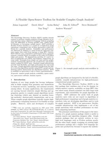
1G1stFron6er2fin114751276777777 rootfi i1415new711111113 114 162ndFron6er11111113foutparents111 345 45newold47775 KDT by “batching” the sparse vectors for the searchesinto a single sparse matrix and using the sparse matrixmatrix multiplication primitive SpGEMM to advance allsearches together. Batching exposes three levels ofpotential parallelism: across multiple searches (columnsof the batched matrix); across multiple frontier verticesin each search (rows of the batched matrix or columns ofthe transposed adjacency matrix); and across multipleedges out of a single high-degree frontier vertex (rows ofthe transposed adjacency matrix). The CombinatorialBLAS SpGEMM implementation exploits all three levelsof parallelism when appropriate.Figure 5: Two steps of breadth-first search, starting4.1.2 The Graph500 Benchmark The intent offrom vertex 7, using sparse matrix-sparse vector multithe Graph500 benchmark [16] is to rank computerplication with “max” in place of “ ”.systems by their capability for basic graph analysis justas the Top500 list [30] ranks systems by capability forfloating-point numerical computation. The benchmarka mini-workflow.measures the speed of a computer performing a BFSon a specified input graph in traversed edges per second4.1 Breadth-First Search(TEPS). The benchmark graph is a synthetic undirectedgraph with vertex degrees approximating a power law,4.1.1 An algebraic implementation of BFSgenerated by the RMAT [24] algorithm. The size of theBreadth-first search (BFS) is a building block of manybenchmark graph is measured by its scale, the base-2graph computations, from connected components tologarithm of the number of vertices; the number of edgesmaximum flows, route planning, and web crawling andis about 16 times the number of vertices. The RMATanalysis [31, 15]. BFS explores a graph starting fromgeneration parameters are a 0.59, b c 0.19, d a specific vertex, identifying the “frontiers” consisting0.05, resulting in graphs with highly skewed degreeof vertices that can be reached by paths of 1, 2, 3, . . .distributions and a low diameter. We symmetrize theedges. BFS also computes a spanning tree, in whichinput to model undirected graphs, but we only counteach vertex in one frontier has a parent vertex from thethe edges traversed in the original graph for TEPSprevious frontier.calculation, despite visiting the symmetric edges as well.In computing the next frontier from the currentWe have implemented the Graph500 code in KDT,one, BFS explores all the edges out of the currentincluding the parallel graph generator, the BFS itself,frontier vertices. For a directed simple graph this isand the validation required by the benchmark specifithe same computational pattern as multiplying a sparsecation. Per the spec, the validation consists of a setmatrix (the transpose of the graph’s adjacency matrix)of consistency checks of the BFS spanning tree. Theby a sparse vector (whose nonzeros mark the currentchecks verify that the tree spans an entire connectedfrontier vertices). The example in Figure 5 discoverscomponent of the graph, that the tree has no cycles,the first two frontiers f from vertex 7 via matrix-vectorthat tree edges connect vertices whose BFS levels differmultiplication with the transposed adjacency matrix G,by exactly one, and that every edge in the connectedand computes the parent of each vertex reached. SpMVcomponent has endpoints whose BFS levels differ by atis KDT’s matrix-vector multiplication primitive.most one. All of these checks are simple to perform withNotice that while the structure of the computaKDT’s elementwise operators and SpMV.tion is that of matrix-vector multiplication, the actualFigure 6 gives Graph500 TEPS scores for both KDT“scalar” operations are selection operations not additionand for a custom C code that calls the Combinatorialand multiplication of real numbers. Formally speaking,BLAS engine directly. Both runs are performed on thethe computation is done in a semiring different fromHopper machine at NERSC, which is a Cray XE6. Each( , ). The SpMV user specifies the operations used toXE6 node has two twelve-core 2.1 Ghz AMD Opteroncombine edge and vertex data; the computational enprocessors, connected to the Cray Gemini interconnect.gine then organizes the operations efficiently accordingThe C portions of KDT are compiled with GNUto the primitive’s well-defined memory access pattern.C compiler v4.5, and the Python interpreter isIt is often useful to perform BFS from multipleversion 2.7. We utilized all the cores in each node duringvertices at the same time. This can be accomplished in625933Copyright SIAM.Unauthorized reproduction of this article is prohibited.

GTEPS!76543210Core GLKDTPBGLKDTScale 193.88.98.933.8Problem SizeScale 22 Scale 37.5327.6473.4Number of cores!Figure 7: Performance comparison of KDT and PBGLbreadth-first search. The reported numbers are inFigure 6: Speed comparison of the KDT and pure MegaTEPS, or 106 traversed edges per second. TheCombBLAS implementations of Graph500. BFS was graphs are Graph500 RMAT graphs as described in theperformed on a scale 29 input graph with 500M vertices text.and 8B edges. The units on the vertical axis areGigaTEPS, or 109 traversed edges per second. Thesmall discrepancies between KDT and CombBLAS are ory, and that in distributed memory KDT exhibits rolargely artifacts of the network partition granted to the bust scaling with increasing processor count.job. KDT’s overhead is negligible.4.2 Betweenness Centrality Betweenness centrality (BC) [14] is a widely accepted importance measurefor the vertices of a graph, where a vertex is “important”the experiments. In other words, an experiment on p if it lies on many shortest paths between other vertices.cores ran on dp/24e nodes. The two-dimensional parallel BC is a major kernel of the HPCS Scalable SyntheticBFS algorithm used by Combinatorial BLAS is detailed Compact Applications graph analysis benchmark [1].elsewhere [9].The definition of the betweenness centrality CB (v)We see that KDT introduces negligible overhead; of a vertex v isits performance is identical to CombBLAS, up to smallX σst (v)discrepancies that are artifacts of the network partition (4.1),CB (v) σstgranted to the job. The absolute TEPS scores ares6 v6 t Vcompetitive; the purpose-built application used for theofficial June 2011 Graph500 submission for NERSC’s where σst is the number of shortest paths betweenHopper has a TEPS rating about 4 times higher (using vertices s and t, and σst (v) is the number of those8 times more cores), while KDT is reusable for a variety shortest paths that pass through v. Brandes [6] gavea sequential algorithm for BC that runs in O(ne) timeof graph-analytic workflows.We compare KDT’s BFS against a PBGL BFS on an unweighted graph with n vertices and e edges.implementation in two environments. Neumann is a This algorithm uses a BFS from each vertex to find theshared memory machine composed of eight quad-core frontiers and all shortest paths from that source, andAMD Opteron 8378 processors. It used version 1.47 then backtracks through the frontiers to update a sumof the Boost library, Python 2.4.3, and both PBGL of importance values at each vertex.The quadratic running time of BC is prohibitive forand KDT were compiled with GCC 4.1.2. Carver is anIBM iDataPlex system with 400 compute nodes, each large graphs, so one typically computes an approximatenode having two quad-core Intel Nehalem processors. BC by performing BFS only from a sampled subset ofCarver used version 1.45 of the Boost library, Python vertices [3].KDT implements both exact and approximate BC2.7.1, and both codes were compiled with Intel C compiler version 11.1. The test data consists of scale by a batched Brandes’ algorithm. It constructs a batch19 to 24 RMAT graphs. We did not use Hopper in of k BFS trees simultaneously by using the SpGEMMthese experiments as PBGL failed to compile on the primitive on n k matrices rather than k separate SpMVoperations. The value of k is chosen based on problemCray platform.The comparison results are presented in Figure 7. size and available memory. The straightforward KDTWe observe that on this example KDT is significantly code is able to exploit parallelism on all three levels:faster than PBGL both in shared and distributed mem- multiple BFS starts, multiple frontier vertices per BFS,626934Copyright SIAM.Unauthorized reproduction of this article is prohibited.

chain, beginning by initializing vertex probabilitiesP0 (v) 1/n for all vertices v in the graph, where nis the number of vertices and the subscript denotes theiteration number. The algorithm updates the probabilities iteratively by (4.2)75Pk 1 (v) 1 d dnXu Adj (v)Pk (u), Adj (u) 50250149163664121256Number of CoresFigure 8: Performance of betweenness centrality inKDT on synthetic power-law graphs (see Section 4.1.2).The units on the vertical axis are MegaTEPS, or 106traversed edges per second. The black line shows ideallinear scaling for the scale 18 graph. The x-axis isin logarithmic scale. Our current backend requires asquare number of processors.and multiple edges per frontier vertex.Figure 8 shows KDT’s performance on calculatingBC on RMAT graphs. Our inputs are RMAT matriceswith the same parameters and sparsity as describedin Graph500 experiments (Section 4.1.2). Since therunning time of BC on undirected graphs is quadratic,we ran our experiments on smaller data sets, presentingstrong scaling results up to 256 cores. We observeexcellent scaling up to 64 cores, but speedup starts todegrade slowly after that. For 256 cores, we see speedupof 118 times compared to a serial run. For all theruns, we used an approximate BC with starting verticescomposed of a 3% sample, and a batchsize of 768. Thisexperiment was run on Hopper, utilizing all 24 cores ineach node.4.3 PageRank PageRank [32] computes vertex relevance by modeling the actions of a “random surfer”. Ateach vertex (i.e., web page) the surfer either traversesa randomly-selected outbound edge (i.e., link) of thecurrent vertex, excluding self loops, or the surfer jumpsto a randomly-selected vertex in the graph. The probability that the surfer chooses to traverse an outboundedge is controlled by the damping factor, d. A typicaldamping factor in practice is 0.85. The output of thealgorithm is the probability of finding the surfer visitinga particular vertex at any moment, which is the stationary distribution of the Markov chain that describes thesurfer’s moves.KDT computes PageRank by iterating the Markovwhere Adj (u) and Adj (u) are the sets of inboundand outbound vertices adjacent to u. Vertices with nooutbound edges are treated as if they link to all vertices.After removing self loops from the graph, KDTevaluates (4.2) simultaneously for all vertices using theSpMV primitive. The iteration process stops when the1-norm of the difference between consecutive iteratesdrops below a default or, if supplied, user-definedstopping threshold .We compare the PageRank implementations whichship with KDT and Pegasus in Figure 9. The datasetis composed of scale 19 and 21 directed RMAT graphswith isolated vertices removed. The scale 19 graph contains 335K vertices and 15.5M edges, the scale 21 graphcontains 1.25M vertices and 63.5M edges and the convergence criteria is 10 7 . The test machine is Neumann (a 32-core shared memory machine, same hardware and software configuration as in Section 4.1.2). Weused Pegasus 2.0 running on Hadoop 0.20.204 and SunJVM 1.6.0 13. We directly compare KDT core countswith maximum MapReduce task counts despite this giving Pegasus an advantage (each task typically shows between 110%-190% CPU utilization). We also observedthat mounting the Hadoop Distributed Filesystem in aramdisk provided Pegasus with a speed boost on the order of 30%. Despite these advantages we still see thatKDT is 2 orders of magnitude faster.Both implementations are fundamentally based onan SpMV operation, but Pegasus performs it via aMapReduce framework. MapReduce allows Pegasus tobe able to handle huge graphs that do not fit in RAM.However, the penalty for this ability is the need tocontinually touch disk for every intermediate operation,parsing and writing intermediate data from/to strings,global sorts, and spawning and killing VMs. Our resultillustrates that while MapReduce is useful for tasks thatdo not fit in memory, it suffers an enormous overheadfor ones that do.A comparison of the two codes also demonstratesKDT’s user-friendliness. The Pegasus PageRank implementation is approximately 500 lines long. It is composed of 3 separate MapReduce stages and job management code. The Pegasus algorithm developer must beproficient with the MapReduce paradigm in addition to627935Copyright SIAM.Unauthorized reproduction of this article is prohibited.

CodePegasusKDTPegasusKDTProblem SizeScale 19Scale 212h 35m 10s 6h 06m 10s55s7m 12s33m 09s 4h 40m 08s13s1m 34sFigure 9: Performance comparison of KDT and PegasusPageRank ( 10 7 ). The graphs are Graph500 RMATgraphs as described in Section 4.1.2. The machineis Neumann, a 32-core shared memory machine withHDFS mounted in a ramdisk.600060Time 21256529Number of Coresthe GIM-V primitive. The KDT implementation is 30lines of Python consisting of input checks and sanitization, initial value generation, and a loop around ourSpMV primitive.Figure 10: Performance of GaBP in KDT on solvinga 500 500 structured mesh, steady-state, 2D heatdissipation problem (250K vertices, 1.25M edges). Thealgorithm took 400 iterations to converge to a relativenorm 10 3 . The speedup and timings are plotted on4.4 Belief Propagation Belief Propagation (BP) is separate y-axes, and the x-axis is in logarithmic scale.a so-called “message passing” algorithm for performing inference on graphical models such as Bayesian networks [37]. Graphical models are used extensively inmachine learning, where each random variable is rep- on Hopper, but we observed similar scaling on theresented as a vertex and the conditional dependencies Neumann shared memory machine.We compared our GaBP implementation withamong random variables are represented as edges. BPcalculates the approximate marginal distribution for GraphLab’s GaBP on our shared memory system. Theeach unobserved vertex, conditional on any observed problem set was composed of structured and unstructured meshes ranging from hundreds of edges to milvertices.Gaussian Belief Propagation (GaBP) is a version of lions. KDT’s time to solution compared favorably withthe BP algorithm in which the underlying distributions GraphLab on problems with more than 10,000 edges.are modeled as Gaussian [5]. GaBP can be used toClustering MarkovClusteringiteratively solve symmetric positive definite systems 4.5 Markovof linear equations Ax b, and thus is a potential (MCL) [36] is used in computational biology tocandidate for solving linear systems that arise within discover the members of protein complexes [13, 7],KDT. Although BP is applicable to much more general in linguistics to separate the related word clusters ofsettings (and is not necessarily the method of choice for homonyms [12], and to find circles of trust in socialsolving a linear equation system), GaBP is often used network graphs [33, 29]. MCL finds clusters by postuas a performance benchmark for BP implementations. lating that a random walk that visits a dense clusterWe implemented GaBP in KDT and used it to solve will probably visit many of its vertices before leaving.a steady-state thermal problem on an unstructuredThe basic algorithm operates on the graph’s adjamesh. The algorithm converged after 11 iterations cency matrix. It iterates a sequence of steps called exon the Schmid/thermal2 problem that has 1.2 million pansion, inflation, normalization and pruning. The exvertices and 8.5 million edges [10].pansion step discovers friends-of-friends by raising theWe demonstrate strong scaling using steady-state matrix to a power (typically 2). Inflation separates low2D heat dissipation problems in Figure 10. The k k and high-weight edges by raising the individual matrix2D grids yield graphs with k 2 vertices and 5k 2 edges. elements to a power which can vary from about 2 to 20,We observed linear scaling with increasing problem higher values producing finer clusters. This has the efsize and were able to solve a k 4000 problem in fect of both strengthening flow inside clusters and weak31 minutes on 256 cores. Parallel scaling is sub- ening it between clusters. The matrix is scaled to belinear because GaBP is an iterative algorithm with column-stochastic by a normalization step.

A Flexible Open-Source Toolbox for Scalable Complex Graph Analysis Adam Lugowskiy David Alberz Ayd n Bulu cx John R. Gilbert{Steve Reinhardtk Yun Teng Andrew Waranisyy Abstract The Knowledge Discovery Toolbox (KDT) enables domain experts to perform complex analyses of huge datasets on su-percomputers using a high-level language without grappling