Transcription
CHAPTER 10DETERMINING HOW COSTS BEHAVE10-11.2.10-21.2.3.The two assumptions areVariations in the level of a single activity (the cost driver) explain the variations in therelated total costs.Cost behavior is approximated by a linear cost function within the relevant range. Alinear cost function is a cost function where, within the relevant range, the graph of totalcosts versus the level of a single activity forms a straight line.Three alternative linear cost functions areVariable cost function––a cost function in which total costs change in proportion to thechanges in the level of activity in the relevant range.Fixed cost function––a cost function in which total costs do not change with changes inthe level of activity in the relevant range.Mixed cost function––a cost function that has both variable and fixed elements. Totalcosts change but not in proportion to the changes in the level of activity in the relevantrange.10-3 A linear cost function is a cost function where, within the relevant range, the graph oftotal costs versus the level of a single activity related to that cost is a straight line. An example ofa linear cost function is a cost function for use of a videoconferencing line where the terms are afixed charge of 10,000 per year plus a 2 per minute charge for line use. A nonlinear costfunction is a cost function where, within the relevant range, the graph of total costs versus thelevel of a single activity related to that cost is not a straight line. Examples include economies ofscale in advertising where an agency can double the number of advertisements for less than twicethe costs, step-cost functions, and learning-curve-based costs.10-4 No. High correlation merely indicates that the two variables move together in the dataexamined. It is essential also to consider economic plausibility before making inferences aboutcause and effect. Without any economic plausibility for a relationship, it is less likely that a highlevel of correlation observed in one set of data will be similarly found in other sets of data.10-51.2.3.4.Four approaches to estimating a cost function areIndustrial engineering method.Conference method.Account analysis method.Quantitative analysis of current or past cost relationships.10-6 The conference method estimates cost functions on the basis of analysis and opinionsabout costs and their drivers gathered from various departments of a company (purchasing,process engineering, manufacturing, employee relations, etc.). Advantages of the conferencemethod include1.The speed with which cost estimates can be developed.2.The pooling of knowledge from experts across functional areas.3.The improved credibility of the cost function to all personnel.10-1
10-7 The account analysis method estimates cost functions by classifying cost accounts in thesubsidiary ledger as variable, fixed, or mixed with respect to the identified level of activity.Typically, managers use qualitative, rather than quantitative, analysis when making these costclassification decisions.10-8 The six steps are1.Choose the dependent variable (the variable to be predicted, which is some type of cost).2.Identify the independent variable or cost driver.3.Collect data on the dependent variable and the cost driver.4.Plot the data.5.Estimate the cost function.6.Evaluate the cost driver of the estimated cost function.Step 3 typically is the most difficult for a cost analyst.10-9 Causality in a cost function runs from the cost driver to the dependent variable. Thus,choosing the highest observation and the lowest observation of the cost driver is appropriate inthe high-low method.10-101.2.3.Three criteria important when choosing among alternative cost functions areEconomic plausibility.Goodness of fit.Slope of the regression line.10-11 A learning curve is a function that measures how labor-hours per unit decline as units ofproduction increase because workers are learning and becoming better at their jobs. Two modelsused to capture different forms of learning are1.Cumulative average-time learning model. The cumulative average time per unit declinesby a constant percentage each time the cumulative quantity of units produced doubles.2.Incremental unit-time learning model. The incremental time needed to produce the lastunit declines by a constant percentage each time the cumulative quantity of unitsproduced doubles.10-12 Frequently encountered problems when collecting cost data on variables included in acost function are1.The time period used to measure the dependent variable is not properly matched with thetime period used to measure the cost driver(s).2.Fixed costs are allocated as if they are variable.3.Data are either not available for all observations or are not uniformly reliable.4.Extreme values of observations occur.5.A homogeneous relationship between the individual cost items in the dependent variablecost pool and the cost driver(s) does not exist.6.The relationship between the cost and the cost driver is not stationary.7.Inflation has occurred in a dependent variable, a cost driver, or both.10-2
10-13 Four key assumptions examined in specification analysis are1.Linearity of relationship between the dependent variable and the independent variablewithin the relevant range.2.Constant variance of residuals for all values of the independent variable.3.Independence of residuals.4.Normal distribution of residuals.10-14 No. A cost driver is any factor whose change causes a change in the total cost of a relatedcost object. A cause-and-effect relationship underlies selection of a cost driver. Some users ofregression analysis include numerous independent variables in a regression model in an attemptto maximize goodness of fit, irrespective of the economic plausibility of the independentvariables included. Some of the independent variables included may not be cost drivers.10-15 No. Multicollinearity exists when two or more independent variables are highlycorrelated with each other.10-16 (10 min.) Estimating a cost function.1.Difference in costsSlope coefficient Difference in machine-hours 5, 400 4,00010,000 6,000 1, 400 0.35 per machine-hour4, 000Constant Total cost – (Slope coefficient Quantity of cost driver) 5,400 – ( 0.35 10,000) 1,900 4,000 – ( 0.35 6,000) 1,900The cost function based on the two observations isMaintenance costs 1,900 0.35 Machine-hours2.The cost function in requirement 1 is an estimate of how costs behave within the relevantrange, not at cost levels outside the relevant range. If there are no months with zero machinehours represented in the maintenance account, data in that account cannot be used to estimate thefixed costs at the zero machine-hours level. Rather, the constant component of the cost functionprovides the best available starting point for a straight line that approximates how a cost behaveswithin the relevant range.10-3
10-17 (15 min.) Identifying variable-, fixed-, and mixed-cost functions.1.See Solution Exhibit 10-17.2.Contract 1: y 50Contract 2: y 30 0.20XContract 3: y 1Xwhere X is the number of miles traveled in the day.3.Contract123Cost FunctionFixedMixedVariableSOLUTION EXHIBIT 10-17Plots of Car Rental Contracts Offered by Pacific Corp.10-4
10-181.2.3.4.5.6.7.8.9.(20 min.) Various cost-behavior patterns.KBGJNote that A is incorrect because, although the cost per pound eventually equals aconstant at 9.20, the total dollars of cost increases linearly from that pointonward.IThe total costs will be the same regardless of the volume level.LFThis is a classic step-cost function.KC10-19 (30 min.) Matching graphs with descriptions of cost and revenue A step-cost function.It is data plotted on a scatter diagram, showing a linear variable cost function withconstant variance of residuals. The constant variance of residuals implies thatthere is a uniform dispersion of the data points about the regression line.10-20 (15 min.) Account analysis method.1.Variable costs:Car wash labor 260,000Soap, cloth, and supplies42,000Water38,000Electric power to move conveyor belt72,000Total variable costs 412,000Fixed costs:Depreciation 64,000Salaries46,000Total fixed costs 110,000Some costs are classified as variable because the total costs in these categories change inproportion to the number of cars washed in Lorenzo’s operation. Some costs are classified asfixed because the total costs in these categories do not vary with the number of cars washed. Ifthe conveyor belt moves regardless of the number of cars on it, the electricity costs to power theconveyor belt would be a fixed cost.2. 412,000 5.15 per car80,000Total costs estimated for 90,000 cars 110,000 ( 5.15 90,000) 573,500Variable costs per car 10-5
10-21 (20 min.) Account analysis1. The electricity cost is variable because, in each month, the cost divided by the number ofkilowatt hours equals a constant 0.30. The definition of a variable cost is one that remainsconstant per unit.The telephone cost is a mixed cost because the cost neither remains constant in total nor remainsconstant per unit.The water cost is fixed because, although water usage varies from month to month, the costremains constant at 60.2. The month with the highest number of telephone minutes is June, with 1,440 minutes and 98.80 of cost. The month with the lowest is April, with 980 minutes and 89.60. Thedifference in cost ( 98.80 – 89.60), divided by the difference in minutes (1,440 – 980) equals 0.02 per minute of variable telephone cost. Inserted into the cost formula for June: 98.80 a fixed cost ( 0.02 number of minutes used) 98.80 a ( 0.02 1,440) 98.80 a 28.80a 70 monthly fixed telephone costTherefore, Java Joe’s cost formula for monthly telephone cost is:Y 70 ( 0.02 number of minutes used)3. The electricity rate is 0.30 per kw hourThe telephone cost is 70 ( 0.02 per minute)The fixed water cost is 60Adding them together we get:Fixed cost of utilities 70 (telephone) 60 (water) 130Monthly Utilities Cost 130 (0.30 per kw hour) ( 0.02 per telephone min.)4. Estimated utilities cost 130 ( 0.30 2,200 kw hours) ( 0.02 1,500 minutes) 130 660 30 82010-6
10-22 (30 min.) Account analysis method.1.Manufacturing cost classification for 2012:AccountDirect materialsDirect manufacturing laborPowerSupervision laborMaterials-handling laborMaintenance laborDepreciationRent, property taxes, adminTotalTotalCosts(1) 0 948,750% ofTotal CostsThat isVariableFixedVariableVariableCostsCostsCost per Unit(2)(3) (1) (2) (4) (1) – (3) (5) (3) 75,000100%10010020504000 300,000225,00037,50011,25030,00030,00000 633,750 00045,00030,00045,00095,000100,000 315,000 4.003.000.500.150.400.4000 8.45Total manufacturing cost for 2012 948,750Variable costs in 2013:AccountDirect materialsDirect manufacturing laborPowerSupervision laborMaterials-handling laborMaintenance laborDepreciationRent, property taxes, admin.TotalUnitIncrease inVariableVariable Variable CostCost perper UnitCostUnit for Percentagefor 2013per UnitIncrease2012(7)(6)(8) (6) (7) (9) (6) (8) 4.003.000.500.150.400.4000 8.455%1000000010-7 0.200.30000000 0.50 4.203.300.500.150.400.4000 8.95Total VariableCosts for 2013(10) (9) 80,000 336,000264,00040,00012,00032,00032,00000 716,000
Fixed and total costs in 2013:AccountFixedCostsfor 2012(11)Direct materials 0Direct manufacturing labor0Power0Supervision labor45,000Materials-handling labor30,000Maintenance labor45,000Depreciation95,000Rent, property taxes, admin. 100,000Total se inFixed Costs(13) (11) (12) 0000004,7507,000 11,750Fixed Costsfor 2013(14) (11) (13) 00045,00030,00045,00099,750107,000 326,750VariableCosts for2013(15)TotalCosts(16) (14) (15) 336,000 062,00077,00032,000099,7500107,000 716,000 1,042,750Total manufacturing costs for 2013 1,042,7502.Total cost per unit, 2012Total cost per unit, 2013 948,750 12.6575,000 1,042,750 13.0380,000 3.Cost classification into variable and fixed costs is based on qualitative, rather thanquantitative, analysis. How good the classifications are depends on the knowledge of individualmanagers who classify the costs. Gower may want to undertake quantitative analysis of costs,using regression analysis on time-series or cross-sectional data to better estimate the fixed andvariable components of costs. Better knowledge of fixed and variable costs will help Gower tobetter price his products, to know when he is getting a positive contribution margin, and to bettermanage costs.10-8
10-23 (15–20 min.) Estimating a cost function, high-low method.1.The key point to note is that the problem provides high-low values of X (annual roundtrips made by a helicopter) and Y X (the operating cost per round trip). We first need tocalculate the annual operating cost Y (as in column (3) below), and then use those values toestimate the function using the high-low method.Highest observation of cost driverLowest observation of cost driverDifferenceCost Driver:Annual RoundTrips (X)(1)2,0001,0001,000OperatingCost perRound-Trip(2) 300 350AnnualOperatingCost (Y)(3) (1) (2) 600,000 350,000 250,000Slope coefficient 250,000 1,000 250 per round-tripConstant 600,000 – ( 250 2,000) 100,000The estimated relationship is Y 100,000 250 X; where Y is the annual operating cost of ahelicopter and X represents the number of round trips it makes annually.2.The constant a (estimated as 100,000) represents the fixed costs of operating ahelicopter, irrespective of the number of round trips it makes. This would include items such asinsurance, registration, depreciation on the aircraft, and any fixed component of pilot and crewsalaries. The coefficient b (estimated as 250 per round-trip) represents the variable
10-1 CHAPTER 10 DETERMINING HOW COSTS BEHAVE 10-1 The two assumptions are 1. Variations in the level of a single activity (the cost driver) explain the variations in the related total costs. 2. Cost behavior is approximated by a linear cost function within the relevant range. A linear cost function is a cost function where, within the relevant range, the graph of total costs versus the level .