Transcription
3543, Page 1Dynamic Modeling and Performance Analysis of Sensible Thermal EnergyStorage SystemsAustin NASH* , Neera JAINPurdue University,West Lafayette, IN, USAnash@purdue.edu* Corresponding AuthorABSTRACTIn this paper we consider the problem of dynamic performance evaluation for sensible thermal energy storage (TES),with a specific focus on hot water storage tanks. We derive transient performance metrics, from second law principles,that can be used to guide real-time decision-making aimed toward improving demand response. We show how thetransient nature of the metrics can be used not only to influence control variables within the system, but also to mitigateadverse effects of disturbances during operation. To evaluate these metrics in the context of hot water storage tanks, athermal stratification model is needed. We derive a reduced-order model which allows the simulation of tank thermalstratification during all modes of system operation. The proposed performance metrics are analyzed in simulationusing the dynamic tank model. The results highlight key trade-offs captured by the metrics that can be incorporatedinto future optimal control design for sensible TES systems.1. INTRODUCTIONMotivation and Problem Definition: Within thermodynamic processes, waste heat losses occur on a large scale due toequipment inefficiencies and limitations. It has been estimated that anywhere from 20-50% of energy consumption inU.S. industrial applications alone is ultimately released as waste heat (Waste Heat Recovery - Technology and Opportunities in U.S. Industry, 2008; Semkov, Mooney, Connolly, & Adley, 2014). As such, there exists a great opportunityto develop and improve strategies for waste heat recovery. Waste heat recovery is most commonly carried out incentralized power plants through heat recovery steam generators where the thermal energy is immediately used togenerate additional electricity (Giaccone & Canova, 2009). However, with increasing penetration of distributed powergeneration through micro-combined heat and power (micro-CHP) systems, opportunities for waste heat recovery at theresidential scale are growing (Barbieri, Melino, & Morini, 2012). In these systems, the recovered heat is typically usedto heat water that is stored in a hot water storage tank for domestic use. The use of a thermal energy storage (TES)system enables the recovered energy to meet future thermal demand. However, in order to design optimal controlstrategies to achieve demand response, dynamic performance metrics for TES systems are needed.Gaps in Literature: Many researchers have studied the development of efficiency metrics to quantify the performanceof hot water storage tanks using second law-based analyses. Most efforts, however, use finite time exergy-basedmetrics, rather than rate-based, metrics (Han, Wang, & Dai, 2009; Li, 2016; Fernández-Seara, Uhı́a, & Sieres, 2007a,2007b). The disadvantage is that, while these types of metrics give a global perspective of performance which can beused in making offline design decisions, they fail to give an idea of how well energy is being used at any given time foronline decision-making. Few researchers to date have performed thermodynamic optimization of equipment involvinghighly transient processes (Pizzolato, Verda, & Sciacovelli, 2015; Sciacovelli, Verda, & Sciubba, 2015). In order tooptimize performance of a sensible TES in real-time, we desire transient second-law based performance metrics whichcan be used to embed advanced control strategies into system operation.As previously mentioned, a common type of sensible TES system is a hot water storage tank. Dynamic modelingof hot water storage tanks has been studied by numerous researchers (Kleinbach, Beckman, & Klein, 1993; Han etal., 2009). Recently, researchers have also developed control-oriented dynamic models for hot water storage tanks4th International High Performance Buildings Conference at Purdue, July 11-14, 2016
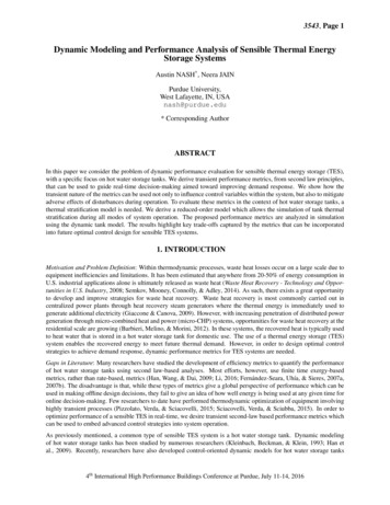
3543, Page 2with simultaneous sink and source mass flow loops (Powell & Edgar, 2013). Many hot water storage tanks utilizean immersed coil heat exchanger as a means of heat absorption, and dynamic models incorporating this feature areavailable within the literature (Cadafalch, Carbonell, Consul, & Ruiz, 2015). However, these models are typicallycomputationally expensive due to the increase in dynamic states that results from the dynamic modeling of the heatexchanger. For eventual control design, we require a reduced-order model of a hot water storage tank with an immersedcoil heat exchanger.Contribution: We define a general set of dynamic performance metrics for the different operation modes of sensibleTES systems. These metrics are then analyzed in simulation using a control-oriented dynamic hot water storage tankmodel; key benefits are demonstrated with respect to real-time decision-making and demand response for hot waterstorage tank operation.Outline: In Section 2 we present a background on performance analysis of TES systems and thermal stratification in hotwater storage tanks. Section 3 describes the sensible TES model proposed in this work, while Section 4 details transientperformance metrics for evaluating system performance. Simulation results demonstrating the dynamic behavior of ahot water storage tank are presented in Section 5, followed by a set of case studies wherein we analyze the performancemetrics developed in Section 4. This is followed by concluding remarks in Section 6.2. BACKGROUNDIn this section, we present an overview on the importance of performance metrics for improving demand response insensible TES systems. We then introduce thermal stratification and its impact on the performance of sensible TES inhot water storage tanks.2.1 Performance Metrics for Sensible Thermal StorageIn electro-chemical batteries, state-of-charge (SOC) is an important concept that enables the control engineer to designalgorithms that effectively utilize the stored electrical energy (Cheng, Divakar, Wu, Ding, & Ho, 2011). In the contextof thermal energy storage, little attention is paid to quantifying SOC; instead, performance and efficiency metricstypically offer a steady-state or aggregate perspective of the behavior of the system (Han et al., 2009; Pizzolato et al.,2015). These steady-state metrics are often used with the intent of influencing offline design factors such as storagesizing. From the perspective of real-time control, we require metrics that not only quantify the current SOC but alsothe charging and/or discharging behavior of the system, so that energy management strategies may be designed andimplemented.2.2 Thermal Stratification in Hot Water Storage TanksThermal stratification in storage tanks is a phenomenon that results when a density gradient is present within the tank.The gradient causes the warmer, less dense water to rise to the top of the tank while the cooler, higher density watersinks to the bottom of the tank. The result is the presence of a high temperature section of water toward the top of thetank and a low temperature section of water at the bottom, as depicted in Fig. 1.In the mixing region between the hot and cold sections, there exists a sharp temperature gradient called a thermocline.Thermal stratification in storage tanks is a very desirable characteristic. It is estimated that the efficiency of the heatstorage can be increased by up to 20% when the tank is kept highly stratified with a thin thermocline region (Hanet al., 2009). Therefore, modeling the dynamic evolution of the thermocline region has important implications onimproving system performance. In order to most accurately quantify the thermal dynamics in a hot water storagetank, partial differential equations are needed in multiple dimensions. Alternatively, a lumped parameter assumptioncan be combined with a spatial discretization in order to derive a one-dimensional (1D) model of the system. A 1Dmodel was introduced in the 1990s (Kleinbach et al., 1993). More recently, Cadafalch et. al. presented a method forincorporating an immersed coil heat exchanger into the analysis (Cadafalch et al., 2015). In the following section, wepresent a control-oriented, reduced-order 1D model for a thermally stratified hot water storage tank with an immersedcoil heat exchanger.4th International High Performance Buildings Conference at Purdue, July 11-14, 2016
3543, Page 3Figure 1: A schematic of a thermally stratified hotwater storage tank.Figure 2: A cylindrical hot water storage tank withan immersed coil heat exchanger.Figure 3: A discretized control volume.Figure 4: Finite difference scheme for discretizednode.3. HOT WATER STORAGE TANK MODELIn this section we present the governing equations for modeling the thermal stratification in a cylindrical hot waterstorage tank. A schematic of the system is shown in Fig. 2. Hot waste heat water at a temperature T in enters animmersed hot water coil situated at the lower portion of the tank. The waste heat water is then pumped verticallythrough the coil until it exits the tank at T out . Heat is transferred from the warm water flowing through the coil to thecolder water in the storage tank. We define three different modes of operation for the system. We define charging tobe the heat addition mode, or the mode during which waste heat water is being pumped through the coil in order toheat the water in the tank. Conversely, we define discharging to be the heat rejection mode, or the mode during whichthe stored hot water is being pumped out of the tank and replaced with cold water. The hot water is removed from thetank at a flow rate ṁt which acts as a disturbance on the system. Moreover, the water in the tank is replenished by anequal flow of water defined as ṁcw which enters at the bottom of the tank. Finally, we define a third mode of operationto be simultaneous charging and discharging of the tank.3.1 Governing EquationsIn this section we derive a control-oriented model of the thermal storage tank dynamics that can be used for modelbased control design. The model presented here builds upon work presented by previous researchers (Kleinbach et al.,1993; Powell & Edgar, 2013; Cadafalch et al., 2015). The tank is discretized vertically into n nodes (Kleinbach et al.,1993), with the top node defined as node one. An illustrative view of a discretized control volume is shown in Fig.3.Each node is allowed to exchange heat with its surroundings in several ways. Nodes can absorb heat from the coil,Q̇coil , and lose heat to the ambient by conduction through the tank walls, Q̇cond,wall . Additionally, each node is allowedto exchange heat with its bordering nodes, modeled as Q̇ j 1 and Q̇ j 1 . While in discharge mode, water flows upwardthrough each control volume. Each node is assumed to remain in steady-state with respect to mass flow. The bottomnode is sized such that it contains the cold water flow inlet valve. Conservation of energy is used to derive a system of4th International High Performance Buildings Conference at Purdue, July 11-14, 2016
3543, Page 4n ordinary differential equations that can be solved numerically, yielding the temperature stratification in the storagetank as a function of time. For the jth node, the energy balance equation ism j cvdT j Q̇coil, j Q̇cond,wall, j Q̇ j 1 Q̇ j 1 ṁt cv (T j 1 T j ) .dt(1)dTOne by one, nodal temperature differentials dt j can be solved independently. Values for heat loss through the walls are Agiven by Q̇cond,wall, j kwallT j T 0 , where kwall is a tuning parameter, wt is the approximate wall thickness, and T 0wtis the temperature of the ambient environment. Logic is used to determine whether each node is within the coil regionwhich in turn dictates whether or not there is heat transfer between the coil and that particular node. The internal heattransfer rate terms Q̇ j 1 and Q̇ j 1 are solved using a finite difference scheme.3.2 Calculation of Internal Heat Transfer Between NodesTo quantify the internal heat transfer rates, Q̇ j 1 and Q̇ j 1 , a finite difference scheme is used (Powell & Edgar, 2013).Fig. 4 helps to illustrate the process. The scheme yields the following expressions for the internal heat transferrates,Q̇ j 1 k j 1 AT j 1 T j,z j 1 z j(2)Q̇ j 1 k j 1 AT j T j 1.z j z j 1(3)The z terms represent heights of the vertical midpoints of the nodes with respect to a zero datum at the tank’s bottom.In Eqns. (2)-(3), the k terms are tuning parameters in the model and are used to handle temperature inversion within themodel (Powell & Edgar, 2013). Temperature inversion is a phenomenon which occurs when warmer, less dense waterexists below cooler, heavier water. In this work, temperature inversion exists due to the presence of the immersed heatcoil in the lower portion of the tank. The coils heat the water at the bottom of the tank; this hot water then rises towardthe top of the tank. One-dimensional models are incapable of naturally accounting for temperature inversion. Hence,an alternative way of incorporating the phenomenon is necessary.At any point in simulation, if the temperature of node j is either lower than the node below or higher than the nodeabove, the k j 1 and k j 1 terms are increased by several orders of magnitude in order to force heat to be transferredupward, thereby resolving the temperature inversion problem. The algorithm for the variation of the coefficients isgiven byk j 1 k j 1 T j T j 1 , if T j T j 1 and k j 1 ,otherwisek j 1 k j 1 T j T j 1 , if T j T j 1 , k j 1 ,otherwise(4)where is a tuning parameter whose magnitude is several orders higher than the magnitude of the k term itself.3.3 Calculation of Coil Heat TransferIn previous work, Cadafalch et. al. present a method of incorporating a transient analysis of the immersed heatexchanger (Cadafalch et al., 2015). In this work, we are interested in a reduced-order model of the interaction betweenthe tank water and the coil in order to obtain a computationally efficient control-oriented model. To calculate the heattransfer rate between the coil and the tank nodes within the coil region, we treat the coil as a separate system actingat steady-state and assume a linear temperature profile from the tank coil inlet to the tank coil outlet as shown in Fig.5.In Fig. 5, the value of T in is known. At any time t, the value of T out is assumed to be equal to the temperature of thewater of the surrounding node. This assumption is based upon the fact that 1) the mass flow rate inside the coil is slow(3-7 liters per minute) and 2) the amount of water in the coil is small in comparison to the overall amount of water inthe tank. Assuming the coil to be at steady-state, the value for the heat transfer rate of the jth coil slice is calculated4th International High Performance Buildings Conference at Purdue, July 11-14, 2016
3543, Page 5Figure 5: Schematic for calculating heat transfer rates due to immersed coil. as Q̇coil, j ṁcoil cv T coil,in, j T coil,out, j . The values for T coil,in, j and T coil,out, j are determined using a linear reduction intemperature from T in at the coil inlet to T out at the coil outlet.4. TRANSIENT PERFORMANCE METRICSIn this section, we present transient second-law based performance metrics for the modes of operation of the hot waterstorage tank.4.1 Charging Performance MeasureTo quantify transient performance during charging mode, we require a metric to compare the rate at which useful work(i.e. exergy) is supplied to the system to the rate at which useful work is lost. Overall, the metric should inform howefficiently exergy is being stored within the system. Therefore, we believe the best way to characterize performanceduring a charging mode is to use the standard exergetic efficiency metric, given byψc 1 Ẋdest,Ẋ sup(5)where Ẋdest represents the total rate of exergy destruction in the tank, Ẋ sup represents the total rate of exergy beingsupplied to the tank, and the subscript c denotes charging. The supplied exergy rate is calculated based on the rate atwhich exergy is transferred via heat transfer from the immersed coil to the tank water. Within each node in the coilregion, there is some amount of exergy transfer via heat transfer. The total rate of supplied exergy to the system isdefined as the summation of all nodal supplied exergy rates as shown in Eqn. (6).Ẋ sup XjẊ sup, j Xj!To1 Q̇coil, jTj(6)To determine the rate of exergy destruction in the tank, an entropy balance is applied to each node. For the jth node,the entropy accounting equation is given byX Q̇i, jdSj ṁt (s j 1 s j ) Ṡ gen, j .dtT b,ii(7)For the heat transfer terms, boundary temperatures are taken to be as given in Table 1. The left hand side of Eqn. (7)is rearranged to yielddS j m j cv dT j ·.dtTjdt4th International High Performance Buildings Conference at Purdue, July 11-14, 2016(8)
3543, Page 6Table 1: Boundary temperatures for heat transfer rates in entropy accounting equationBoundary temperatureHeat transfer termQ̇coil, jQ̇ j 1Q̇ j 11212Q̇cond,wall, j Tj T j T j 1 T j T j 1ToEquation (7) can be solved for Ṡ gen, j . Then the corresponding exergy destruction rate for the jth node is Ẋdest, j T o Ṡ gen, j . The total rate of exergy destruction in the tank is found by summing all of the nodal exergy destruction rates:PẊdest j Ẋdest, j .4.2 Discharging Performance MeasureFor any mode involving a discharge of thermal energy, we seek to quantify performance by analyzing the rate at whichuseful work is being recovered relative to the rate at which the stored thermal energy is changing. We define thedisharge performance metric to beψd Ẋrec,Ẋ sto(9)where Ẋrec is the rate at which exergy is being recovered from the TES, Ẋ sto is the rate at which exergy is being stored,and the subscript d denotes a discharging mode. In order to determine the rate at which exergy is stored, exergyaccounting equations are used on each node. For the jth node, the rate of change of exergy is given by!XdToQ̇i, j ṁt (x j 1 x j ) T o Ṡ gen, j ,Xj 1 dtT b,ii(10)where the boundary temperatures correspond to those given in Table 1 and Ṡ gen, j is calculated according to Eqn. (7).We define the total rate of exergy stored in the system to beẊ sto X dX jjdt.(11)We define the rate of exergy recovered during discharge to be the rate of flow exergy exiting the top of the tank withrespect to a setpoint state whose temperature is T set . The setpoint state acts as a threshold for undesirable systemperformance during a discharging mode. We take the rate of recovered exergy to be"!#T1Ẋrec ṁt (x1 x set ) ṁt cv (T 1 T set ) T o cv ln.T set(12)The value of T set is a user-defined parameter which serves to quantify the instant at which useful work is no longerbeing recovered from the system. Once the temperature of the water at the top of the storage, T 1 , is less than T set , therecovery rate will become a negative quantity, thereby changing the sign of the performance metric.5. SIMULATION RESULTSIn this section, we first present the dynamic evolution of tank thermal stratification during the simultaneous chargingand discharging operation mode. Next, we demonstrate how the dynamic performance metrics capture the relative4th International High Performance Buildings Conference at Purdue, July 11-14, 2016
3543, Page 7effect of control input variables and disturbance input variables on system performance using the dynamic storagetank model. The physical parameters used in these simulation studies are based on an experimental micro-CHPsystem at Purdue University; values are provided in Table 2. A discretization of 30 nodes is used in all simulationstudies, yielding 30 dynamic states.Table 2: Baseline values used for hot water storage tank model simulationsParameterValueParameterValuetank heighttank diametercoil inlet temperaturedead state temperaturetake initial temperaturecold water supply temperature1.3 m0.4 m45 C20 C20 C20 Ccoil volumetric flow ratetank volumetric flow ratetank wall thicknessheight of coil inletheight of coil outletset point temperature2 lpm2 gpm0.051 m0.15 m0.58 m30 C5.1 Dynamic Thermal Stratification BehaviorThe tank is initially charged for two hours. During this time, hot waste heat water from an integrated power generationsystem flows through the coil, thereby exchanging heat with the tank. At t 120 minutes, the tank enters thesimultaneous charging/discharging mode in which hot water is removed from the tank at a specified flow rate ṁd whileheat continues to be added to the system by the coil. The temperature evolution of the thermal stratification for thismode, over a period of 30 minutes, is shown in Fig. 6.(a) minute 130(b) minute 140(c) minute 150Figure 6: Illustration of thermal stratification during 30 minute simultaneous charge/discharge.In Fig. 6a, the charge/discharge has been ongoing for ten minutes. A portion of the hot water above the coil region hasexited the tank and been replenished with the cold water supply. However, the coil waste heat water continues to heatthe cold water as it is drawn upwards through the tank. In Fig. 6b, it is clear that the hottest water in the tank, whichwas located above the coil at a temperature of 40 C, has been removed from the tank. Finally, in Fig. 6c, all of thewater above the coil region is at a temperature below 30 C. At this point, the tank has reached its steady-state thermalgradient; water being removed from the tank is heated from the cold water supply temperature of 20 C to about 27 Cbefore it leaves the tank. The mixing of the water being heated by the coil, and the cold supply water flowing into thetank, results in a widened thermocline.5.2 Analyzing System PerformanceIn this section, we present results for performance characterization of the different modes of system operation. Performance is analyzed with respect to two types of variables: (1) control variables and (2) disturbance variables.4th International High Performance Buildings Conference at Purdue, July 11-14, 2016
3543, Page 85.2.1 Control Variables and Charging Performance Within the system, one variable over which we have controlauthority is the volumetric flow rate of hot waste heat water through the immersed coil. In order to examine thecharging performance of the system, a three hour charge is simulated for coil flow rates varying from one to five litersper minute (lpm). In each case, charging performance is quantified according to Eqn. (5) and the results are comparedin Fig. 7.(a) first 30 minutes(b) full 3 hoursFigure 7: Simulation results depicting effect of varying coil flow rate on charge performance.Figure 7(a) shows that initially, higher flow rates yield better performance. However, as times progresses, the higherflow rates actually have an adverse effect on system performance. As the tank heats up, there is a decrease in thetemperature differential between the waste water in the coil and the water in the tank. This leads to a decrease inthe heat transfer rate between the coil and the tank, and consequently, there is less useful work being supplied to thetank. This aspect of system performance can be seen more clearly through Fig. 8 which shows how the coil outlettemperature varies as a function of time. Based on the assumptions presented in Section 3, the coil outlet temperatureat any time is equal to that of the surrounding water in the tank. In Fig. 8, we see that for high coil flow rates, thetank heats up, or charges, more quickly. However, the tank then reaches its maximum state of charge more quickly aswell, and system performance subsequently degrades as the coil cannot add any additional charge to the system. Oncethe maximum charge is reached, a higher amount of useful work is lost relative to the amount being supplied via theimmersed heat exchanger coil.Figure 8: Simulation results depicting effect of varying coil flow rate on coil outlet temperature.Figure 9: Simulation results depicting effect of varying tank flow rate on discharge performance.These results suggest that in order to maximize the charging rate while also maximizing charging efficiency, a variablecoil flow rate could be used. For example, the coil flow rate could be set high toward the beginning of the chargingperiod but later decreased as the derivative of the efficiency curve becomes negative. In this way, the performance4th International High Performance Buildings Conference at Purdue, July 11-14, 2016
3543, Page 9metric for charging modes can be used in real-time to make control decisions to help improve global system performance.5.2.2 Disturbance Variables and Discharging Performance From a controls perspective, we are also interested inunderstanding the effect of measured disturbances on system performance. The primary disturbance input is thevolumetric flow rate of water exiting the tank during a discharge mode. While we cannot control the timing or durationof discharge modes, we can use the performance metric in Eqn. (9) to inform real-time control decisions in order tolimit adverse effects from an energy utilization standpoint.To investigate the effects of different discharge flow rates on the system, we charge the tank from its cold state fortwo hours. The hot waste heat water is then turned off and a discharge mode is allowed to commence for 30 minutesat a specified tank flow rate. Fig. 9 compares the discharge performance for tank flow rates ranging from one to fivegallons per minute, or 3.8-11.4 lpm. The figure shows that higher tank flow rates allow better performance at first.However, as the state-of-charge decreases, performance at higher flow rates degrades quickly. This makes intuitivesense; as hot water is removed from the tank, cold supply water is being added to the tank thereby reducing the overallstate-of-charge. This is further illustrated by Fig. 10.(a) exergy available in tank(b) rate of change of available exergyFigure 10: Simulation results depicting effect of varying tank flow rate on exergy storage rate and availablestorage.In Fig. 10b, we see that for higher flow rates, the absolute value of the rate of change of exergy, dXdt , or the exergystorage rate, quickly decreases. The result is that the available exergy within the system decreases rapidly, seen in Fig.10a. As the high flow rates deplete the system of its charge, cold water is pumped into the system and the availablethermal energy decreases further. The system rapidly approaches steady state in which cold water exists uniformlythroughout the tank and useful work is unavailable. For smaller tank flow rates, the exergy storage rate in the systemdecreases much less rapidly, signaling that a higher amount of charge remains available within the storage. Thesimulations presented in this section allow real-time insight into system performance for various modes of operation.Performance metrics can be used to design control algorithms aimed at improving demand response and to mitigateadverse effects on performance with respect to disturbances.6. CONCLUSIONIn this paper we defined a set of dynamic performance metrics that are generalizable to a range of thermal energystorage systems. These metrics were then analyzed in the context of a hot water storage tank with an immersed coilheat exchanger, a common type of sensible TES system. We derived a reduced-order model for simulating thermalstratification within the hot water storage tank. More specifically, a simplified model for the interaction between thetank’s immersed coil heat exchanger and the surrounding water reduced the overall number of dynamic states neededto describe the transient behavior of the system. Using the dynamic hot water storage tank model, we demonstrated4th International High Performance Buildings Conference at Purdue, July 11-14, 2016
3543, Page 10the sensitivity of the performance metrics to changes in both control input variables and disturbance input variables.The performance metrics presented for each mode of operation will enable future work aimed at designing advancedcontrol algorithms for improved system performance and demand response.NOMENCLATUREAcvkṁψQ̇areaspecific heatheat transfer coefficientmass flow rateperformance metricheat transfer ratesTwtxzentropytemperaturetank wall thicknessspecific exergyheight in tankSubscriptbboundarycchargeddischargedest destroyedgen generatedjj 1j 1supt0node jnode above jnode below jsuppliedtankdead stateREFERENCESBarbieri, E. S., Melino, F., & Morini, M. (2012, September). Influence of the Thermal Energy Storage on theProfitability of Micro-CHP Systems for Residential Building Applications. Applied Energy, 97, 714–722.Cadafalch, J., Carbonell, D., Consul, R., & Ruiz, R. (2015, February). Modelling of Storage Tanks with ImmersedHeat Exchangers. Solar Energy, 112, 154–162.Cheng, K. W. E., Divakar, B. P., Wu, H., Ding, K., & Ho, H. F. (2011, January). Battery-Management System (BMS)and SOC Development for Electrical Vehicles. IEEE Transactions on Vehicular Technology, 60(1), 76–88.Fernández-Seara, J., Uhı́a, F. J., & Sieres, J. (2007a, January). Experimental Analysis of a Domestic Electric HotWater Storage Tank. Part II: Dynamic Mode of Operation. Applied Thermal Engineering, 27(1), 137–144.Fernández-Seara, J., Uhı́a, F. J., & Sieres, J. (2007b, January). Experimental Analysis of a Domestic Electric HotWater Storage Tank. Part I: Static Mode of Operation. Applied Thermal Engineering, 27(1), 129–136.Giaccone, L., & Canova, A. (2009, June). Economical Comparison of CHP Systems for Industrial User with LargeSteam Demand. Applied Energy, 86(6), 904–914.Han, Y., Wang, R., & Dai, Y. (2009, June). Thermal Stratification Within the Water Tank. Renewable and SustainableEnergy Reviews, 13(5), 1014–1026.Kleinbach, E., Beckman, W., & Klein, S. (1993). Performance Study of One-dimensional Models for StratifiedThermal Storage Tanks. Solar Energy, 50(2), 155–166.Li, G. (2
3.HOT WATER STORAGE TANK MODEL In this section we present the governing equations for modeling the thermal stratification in a cylindrical hot water storage tank. A schematic of the system is shown in Fig. 2. Hot waste heat water at a temperature T in enters an immersed hot water coil situated at the lower portion of the tank.