WIXLIB

FeatureSea Ice ConcentrationSurface Pressure10m Wind SpeedNear-Surface Humidity2m Air TemperatureShortwave RadiationLongwave RadiationRain RateSnow RateSea Surface ERA5ERA5Units% per 350Table 3.1: Input Features for CNN and ConvLSTM models. All features are monthly-averaged and one-month lagged.sea ice. Studies have also shown that Arctic circulation and wind patterns have seasonally varyingrelationships with sea ice [10, 17]. For example, poleward winds specifically play a key role intransporting heat to the Arctic, which contributes to ice melt [2,21,35]. Precipitation trends are alsoconnected to sea ice patterns. In recent years, earlier rainfalls during spring have triggered earliersnowmelt and, via feedback loops, earlier Arctic ice melt [11, 26]. The complexity of atmospheric,oceanic, and sea ice interactions is illustrated in [16, 18], which highlights the pathway by whichregional differences in atmospheric pressure facilitate increased Arctic humidity, which in turnenables higher levels of longwave radiation to reach the sea surface, leading to earlier melting ofsea ice. Thus, each predictor impacts Arctic sea ice through complex physical interactions in theocean and atmosphere.3.1Data ExplorationTo begin our background research, we created climatologies and anomalies to visualize andanalyze the dataset. We calculated the average sea ice extent for each month from 1979 through2018, shown in Fig. 3.1. With this data, we were then able to calculate anomalies in specific yearsto identify years where sea ice extent was substantially lower than the average of all of the years ofdata used. In performing anomaly calculations of sea ice, we were able to see that 2012 had recordlow sea ice extent values (Fig. 3.2). Although the anomalies only reach a 6% difference from themonthly averages, it must be noted that the monthly averages were calculated over a 40 year timeperiod where sea ice extent has changed dramatically. Knowing this, we can better identify theextremes that such anomaly values indicate.With this information, we were able to further analyze which variables could have the largestimpact on sea ice extent. One variable that seems to correlate the most with low sea ice extentis T2m values (Fig. 3.3). Along with related research that shows the affects of temperature onSIE [30], Figure 3.3 shows much higher temperatures 2 meters above sea surface level occurringin summer months, which can be correlated to the decline in SIE in September. This correlation,however, is not as evident in other variables such as sea surface temperature (SST). Although SSTdoes correlate with the changes in our climate and can affect sea ice extent, it does not have asstrong of an impact as other factors such as T2m.Time series analysis was conducted to provide baseline models for comparison with our deeplearning results. By using Seasonal Autoregressive Integrated Moving Average (SARIMA), we wereable to build a forecasting model based on time series seasonality of sea ice concentration. Ourmodel predicted future average sea ice concentration, but the results were not promising. Not only4

Figure 3.1: Monthly averaged sea ice extent values from 1979-2018 were averaged together grouping by month to create a 40 year climatology representingsea ice extent percentage values. These values were further used in calculating sea ice extent anomalies.Figure 3.2: Plot of anomalies created by averaging monthly values of sea ice concentration from 1979-2018 and subtracting those values from the averagemonthly sea ice extent values for 2012 resulting in 12 total anomaly values measured by percentage of sea ice concentration.did the model produce negative values, but it also strongly underestimated the Arctics freezingseasons.Along with using SARIMA, we forecasted sea ice extent using a Vector Autoregression (VAR)model. This statistical model captures the fluctuations and changes in data over time. VARproved to be fairly accurate in comparison to SARIMA. Results showed a basic understanding ofthe changes in sea ice extent averages through seasons but seemed to struggle when calculatingmaximums and minimums in the time series (Fig. 3.4).The purpose of doing this analysis prior to implementing deep learning techniques was to get anunderstanding of the data we were working with. By plotting changes in the data and running thedata through time series analysis, we were able to understand seasonal changes in the data and gainknowledge that would be useful in further analyzing results produced in the deep learning models.Knowing seasonality changes along with the basic structure of the data proved to be essential introubleshooting our later deep learning work.5

Figure 3.3: Plot of anomalies created by averaging monthly values of T2m from 1979-2018 and subtracting those values from the average monthly T2m valuesfor 2012 resulting in 12 total anomaly values.After completing the time series analysis we were able to implement deep learning techniquesin our data, building neural networks in order to predict future sea ice extent.3.2Data PreprocessingAll variables were averaged from a daily resolution to the monthly scale. Prior to model-specificpre-processing, the dataset had 504 images, each with 448 by 304 grid cells and 10 channels,corresponding to the 10 input features details in Table 3.1.3.3Convolutional Neural Network Data PrepreocessingCNN models were trained on the first 407 months of the data (January 1979 - November2012) and validated on the last 96 months (January 2013 - November 2020), with a one-monthlead time. Each image in the dataset was considered to be an individual training example andwas used to predict per-pixel sea ice concentrations for the next month. For example, the imagecorresponding to January 1979 was used to predict ice concentrations for February 1979. Thus,the training dataset learned per-pixel sea ice concentrations for February 1979 - December 2012,and the validation dataset predicted per-pixel sea ice concentrations for February 2013 - December2020.3.4Convolutional LSTM Data PreprocessingIn order to fully capture the spatio-temporal nature of our data using a Convolutional LSTM,heavy data preprocessing was necessary. The model was trained on the first 408 months of thedata and validated on the last 95 months of the data. In Keras, ConvLSTM2D layers require 5dimensional inputs of shape (samples, timesteps, rows, columns, features). To reshape the data,a stateless rolling window was applied to the training and testing data, creating 396 samples of12 months each. Sample one contained months 1-12, sample two contained months 2-13, and thelast sample contained months 395-407. The final shape of the training input data was 396 sampleswith 12 months of 448 304 pixel images, each containing 11 feature measurements at each pixel.6

Figure 3.4: VAR model forecast vs actual values for variables; ice extent, shortwave radiation, longwave radiation, rain, surface pressure, humidity, seasurface temperature, temperature, wind, and snow.Similarly, the final shape of the test input data was 84 samples with 12 months of 448 304 pixelimages each, all containing 11 feature measurements at each pixel.The validation data consisted of 396 images in the training set and 84 images in the test set.Each image contained the average sea ice concentration for the corresponding month in each pixel.The first sample of input data, consisting of the first 12 months of images, was used to predict thesea ice concentrations in the 13th month in the output data; the second sample was used to predictthe SIC in the 14th month.Including a rolling window with 12-month timesteps allowed the ConvLSTM to learn yearlyvariations and relationships in SIC, resulting in more accurate predictions.7

44.1MethodsMasked Loss FunctionNeural networks use loss functions to measure the error in their predictions after each epoch.Once the error has been measured, the model optimizes the loss function using a process calledback-propagation.To help the model learn on ocean and ice pixels while ignoring land pixels, a custom loss functionwas implemented in the networks’ architectures. A land mask was applied to each output of thenetwork before loss was evaluated. In the mask, land pixels were given a value of 0 and non-landpixels were given a value of 1. Each predicted output and the mask were multiplied elementwise,resulting in land pixels being ignored when calculating the loss.After applying the mask, the root mean squared error of the model’s predicted and actual valueswas calculated. By applying land masks, the model learned to ignore land pixels in its calculations,allowing it to more accurately optimize sea ice concentrations for non-land pixels.4.2Convolutional Neural NetworkCNNs are a type of deep learning model particularly suited for working with images, speech,and audio signals. Thus, we chose to implement it to process our per-pixel data, which is in theform of image data. CNNs are able to process multidimensional data. In our case, the input is athree-dimensional array, i.e., height width channel (448, 304, 11). CNNs consist of three typesof layers: convolutional layers, pooling layers, and fully connected layers [12]. We will explain eachlayer type below in detail.Convolutional layers are where the majority of computation is done. In this layer a small matrixof fixed weights, aka a kernel, is passed over an image to create a feature map of the image usingthe following equation:g(x, y) ω · f (x, y) aXbXω(dx, dy)f (x dx, y dy)(4.1)dx a dy bWhere g(x, y) is the feature map, w(dx, dy) is the kernel, and f (x, y) is the original image. Firstthe kernel is applied to an area of the image, where the dot product of the input pixels and thefilter are fed into an output array. Afterwards, the filter shifts by a stride, repeating the processuntil the kernel has swept across the entire image and created a feature map [33]. This allows themodel to recognize patterns such as edges or curves which recur through the image.Pooling layers are used for reducing the amount of parameters in the input. Similar to convolutional layers, pooling layers sweep a small matrix across the image; however this matrix does notcontain weights, it instead applies an aggregation function to the values within the receptive field.The two types of pooling layers are max pooling and average pooling. Max pooling simply choosesthe pixel in the receptive field with the maximum value and sends it to the output array. Averagepooling calculates the average value within the receptive field as it moves across the image to sendto the output array.Fully connected layers connect output layers to nodes of the previous layer. The input image isnot directly connected to the output.The purpose of this CNN is to predict spatial average sea ice concentration per month usingvariable measures across all longitudes and latitudes as input. With the input of different variables and historic sea ice data, the model will produce predictions for monthly averaged sea iceconcentrations in the Arctic.8

Figure 4.1: CNN model architecture.4.3Convolutional Long Short Term Memory NetworkConvLSTM architecture combines the spatial recognition capabilities of convolutional neuralnetworks and the temporal modeling capabilities of long short-term memory models (LSTM) toproduce an output which takes spatial and temporal patterns into account. LSTMs use matrixmultiplication on each gate in an LSTM cell; ConvLSTMs replace this matrix multiplication withconvolutions, allowing the model to capture underlying spatial features in multi-dimensional data[13].By combining convolutions and LSTM gates, a ConvLSTM is able to capture both spatial andtemporal patterns in our data. Values for each of the ConvLSTM gates are calculated using thefollowing equations:ct ft Ct 1 it tanh(Wxc xt Whc ht 1 bc )(4.2)it σ(Wxi xt Whi ht 1 Wci ct 1 bi )(4.3)ft σ(Wxf Xt Whf ht 1 Wcf ct 1 bf ),(4.4)ot σ(Wxo xt Who ht 1 Wco ct bo )(4.5)ht ot tanh(ct )(4.6)where represents a convolution and represents a Hadamard transformation.The structure of ConvLSTM networks is nearly identical to the structure of LSTM networks;however, ConvLSTM networks utilize 3D tensors for gates, inputs, and outputs. ConvLSTMsinclude memory cells, represented as ct in Equation 4.2, which are modified by certain gates. Theinput gate, it in Equation 4.3, allows the memory cell to accumulate information. The forget gate,Ft in Equation 4.4, allows the memory cell to disregard the past cell status, ct 1 . The output gate,9

Ot in Equation 4.5, controls whether the latest memory cell value will be fed to the node’s finalstate, ht in Equation 4.6 [14].Similar to the CNN, the ConvLSTM will predict monthly averaged SIC over all longitudes andlatitudes. The main difference in the ConvLSTM is the addition of temporality to the spatial inputswhich produce monthly outputs that represent the prediction for Arctic sea ice concentration.4.4Multi-Task ModelsMulti-task learning is a subset of machine learning where multiple tasks are learned by a sharedmodel [8]. Our network was trained to produce monthly image predictions of SIC for each pixelwhile also predicting a single sea ice extent value.4.4.1Multi-Task ConvLSTM and CNNBoth the CNN and ConvLSTM also feature multi-task learning. A branched architecture isimplemented to allow the model to learn on multiple tasks. The models contain a shared root,where data is input, and two subsequent branches which produce the SIC image and sea ice extentoutputs. The input root for the ConvLSTM consists of one ConvLSTM2D layer with 8 filters ofsize 5 5 and ReLU activation, followed by two alternating max pooling and convolution layers.The only difference for the CNN is that the first layer is a convolutional layer; everything elsethat follows replicates the architecture of the ConvLSTM. The max pooling layers contain filtersof size 4 4, while the convolutional layers contain 128 and 32 size 5 5 filters respectively. Theconvolutional layers use ReLU activation. The data is then flattened and propagated through adense layer with 256 nodes and ReLU activation.The image branch of the architecture receives the model’s root output and propagates it througha dense layer of size 448 304 136192 with linear activation. The data is then reshaped intoan image of size 448 rows 304 columns. Each pixel in the image contains an SIC measurement,scaled as a percentage out of 100.The extent branch also receives the model’s root output; it propagates the root output vectorthrough 4 dense layers of size 128, 32, 8, and 1 respectively, returning a single sea ice extent resultfor each input sample. The first 3 dense layers include a ReLU activation function, while the outputlayer utilizes linear activation for regressionTwo equally weighted loss functions are used to optimize the models. The image branch isoptimized using the custom masked loss function described in section 4.1, while the sea ice extentbranch is optimized using MSE loss. The performance of the models are evaluated using the RMSEmetric for both branches.4.5Post-Processed ResultsDue to results producing outlier values when running both the ConvLSTM and CNN withand without the multi-task implementation, post-processing was utilized to create more accurateresults. The main aspects of this study’s post processing were: removing values below zero andabove 100, setting a mask for land and open ocean values, and dealing with missing values in theNorth Pole Hole.Values below 0 were set to 0 and values above 100 were set to 100. This step was necessary asthe model results contained considerable noise in areas surrounding sea ice, while also increasingthe amount of ice in heavier concentrations. After post-processing the data to ignore the noise,results showed strong cohesion with actual values and produced much lower RMSE values.10

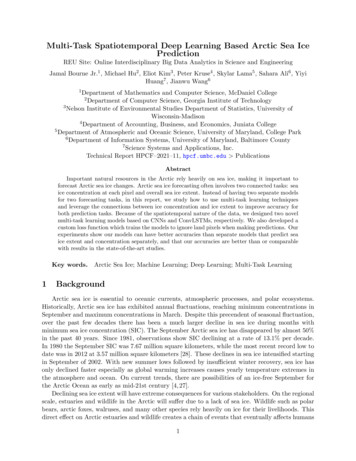
By adding a mask to the predicted SIC values over land, noise in areas without ice were furthereliminated. The mask works by multiplying values over land pixels by 0 and values over sea pixelsby 1 in order for results to only focus on sea ice values rather than outliers that were skewing theaccuracy.The last aspect in post-processing to note was filling the North Pole Hole. The North Pole Holeis a region in the Arctic where satellite imagery does not produce observations. Because of this holein the data, either filling it with interpolated values or leaving it as zero produced inaccurate resultsas the model learned data that is not observed in the actual data. Instead, in post processing, thenorth pole hole was recognized as NaN values so that the model simply ignored the area.5ResultsIn comparing results from this study’s two models, RMSE and NRMSE were used to analyze which models had better accuracy. RMSE and NRMSE were calculated using the followingequations:vu nuX (yˆi yi )2RM SE t(5.1)Ni 1RM SE(5.2)ȳAnother factor to note in comparing the models is that they are all trained on the years 19792012 and tested from 2013-2020. More information on this can be found in Section 3.2 whichdiscusses data preprocessing.N RM SE 5.1CNNFigure 5.1: CNN derived predicted vs. Actual SIE values million km2 .The base convolutional neural network attained an RMSE of 12.005% SIC for 2013 through 2020.After post-processing was applied to the predictions, the RMSE decreased to 7.106%. Implementing11

SIE loss in conjunction with SIC loss for the CNN resulted in a small improvement in SIC prediction.While the test RMSE increased to 12.228%, the post-processed test RMSE fell to 6.993%, the lowestSIC RMSE among all models.Sea ice extent values were calculated from the predicted SIC images of the base CNN and extentloss CNN. The base CNN resulted in an extent test RMSE of 0.868 million km2 , a significantimprovement over the baseline VAR model. The extent loss CNN resulted in an extent test RMSEof 0.600 million km2 , a major improvement over the base CNN model. Overall, the extent lossCNN resulted in lower SIC and SIE errors compared to the base CNN, indicating the benefit ofincorporating both SIC and SIE errors in the model loss function.Figure 5.1 shows the predicted SIE values for the extent loss CNN compared to the real SIEvalues for 2013-2020. The model was able to predict the March SIE maxima with a high degree ofaccuracy. However, the model had a significant and consistent overestimate of the September SIEminima.5.2ConvLSTMFigure 5.2: ConvLSTM derived predicted vs. Actual SIE values million km2 .The convolutional LSTM produced an RMSE of 11.478% on image SIC testing data from 2014to to 2020; its NRMSE was 1.116. Af

3Nelson Institute of Environmental Studies Department of Statistics, University of Wisconsin-Madison 4Department of Accounting, Business, and Economics, Juniata College 5Department of Atmospheric and Oceanic Science, University of Maryland, College Park 6Department of Information Systems, University of Maryland, Baltimore County