Transcription
Ann. Geophysicae 15, 1048 1056 (1997) Ó EGS Springer-Verlag 1997A study of atmospheric gravity waves and travelling ionosphericdisturbances at equatorial latitudesR. L. Balthazor, R. J. Mo ettUpper Atmosphere Modelling Group, School of Mathematics and Statistics, University of She eld, She eld S3 7RH, UKReceived: 15 November 1996 / Revised: 4 March 1997 / Accepted: 11 March 1997Abstract. A global coupled thermosphere-ionosphereplasmasphere model is used to simulate a family oflarge-scale imperfectly ducted atmospheric gravitywaves (AGWs) and associated travelling ionosphericdisturbances (TIDs) originating at conjugate magneticlatitudes in the north and south auroral zones andsubsequently propagating meridionally to equatoriallatitudes. A fast' dominant mode and two slower modesare identi ed. We nd that, at the magnetic equator, allthe clearly identi ed modes of AGW interfere constructively and pass through to the opposite hemisphere withunchanged velocity. At F-region altitudes the fast'AGW has the largest amplitude, and when northwardpropagating and southward propagating modes interfere at the equator, the TID (as parameterised by thefractional change in the electron density at the F2 peak)increases in magnitude at the equator. The amplitude ofthe TID at the magnetic equator is increased comparedto mid-latitudes in both upper and lower F-regions witha larger increase in the upper F-region. The ionosphericdisturbance at the equator persists in the upper F-regionfor about 1 hour and in the lower F-region for 2.5 hoursafter the AGWs rst interfere, and it is suggested thatthis is due to enhancements of the TID by slower AGWmodes arriving later at the magnetic equator. Thecomplex e ects of the interplays of the TIDs generatedin the equatorial plasmasphere are analysed by examining neutral and ion winds predicted by the model, andare demonstrated to be consequences of the forcing ofthe plasmasphere along the magnetic eld lines by theneutral air pressure wave.1 IntroductionThe relationship between atmospheric gravity waves(AGWs) and travelling ionospheric disturbances (TIDs)Correspondence to: R. L. Balthazorhas been documented in detail, with notable papers byHines (1960), Hines (1974), Richmond (1978), Hunsucker(1982) and Jing and Hunsucker (1993), and reviewed mostrecently by Hocke and Schlegel (1996). The TID is thesignature in the ionosphere of the passage of the AGW,the ions being forced along the eld lines by the neutral airwinds driven by the pressure wave. Various techniqueshave evolved for studying TIDs such as ionosonde andradar (e.g. Williams et al., 1988; Fukao et al., 1993),satellite (e.g. Johnson et al., 1995) and tomographictechniques (e.g. Pryse et al., 1995), and have cast light onthe validity of theoretical and numerical models (e.g.Millward et al., 1993b; Kirchengast et al., 1996).However, there has been a relative scarcity ofinvestigations of AGWs and TIDs at equatorial latitudes. Ionospheric irregularities at equatorial latitudeshave been examined recently by Hajkowicz (1995) andBowman (1995). These e ects have been previouslyexplained as AGW seeding' of equatorial spread-F(Kelley, 1989). Hocke and Schlegel (1996) review theresults of several observational campaigns, includingthose observing near, at or across the equator (Thome,1968; Sterling et al., 1971; Hajkowicz and Hunsucker1987) and Hajkowicz and Hunsucker (1987) suggestthat, in the case of AGWs and associated TIDsapproaching the equator from both hemispheres, it islikely that both TIDs produce a constructive interference e ect at the points of their encounter near theequator''. Large-scale ionospheric disturbances propagating equatorwards and associated with low-latitudeaurorae have been studied by Igarashi et al. (1991).Satellite measurements (Gross et al., 1984) reveal thepresence of standing waves in the equatorial ionosphere, possibly as a result of interference between waves fromtwo sources (both auroral regions)'' and Hajkowicz(1991) has shown that geomagnetic activity can produceconjugate AGWs travelling from both auroral zones.Fesen et al., (1989) used separate thermospheric andionospheric models to examine the e ects of a geomagnetic storm and showed that the equatorial disturbancesobserved were the result of neutral winds and AGWs.
R. L. Balthazor, R. J. Mo ett: A study of atmospheric gravity waves and travelling ionospheric disturbancesThis study simulates simultaneous ion-velocity burstsin both north and south auroral zones at conjugatemagnetic latitudes. The propagation of the resultantAGWs is examined, with emphasis on the TIDsproduced at equatorial latitudes. The authors note herethat whilst TIDs do not technically propagate' (as theyare the signatures in the ionosphere of the propagatinggravity wave), phrases such as the propagation of theTID' have become embedded in the literature. Whilst wehave taken pains to avoid this inaccuracy, it is perhapsinevitable that such phrases creep into usage. Weemphasise, however, that it is the AGWs that propagate,and the TIDs are merely a signature.2 Model descriptionThe She eld/UCL/SEL global model of the coupledthermosphere ionosphere plasmasphere has previously been described by Millward et al. (1993b) andmore extensively by Fuller-Rowell et al. (1996) andMillward et al. (1996). In brief, coupled equations ofmomentum, energy and continuity are solved at xedgrid points to calculate values of density, temperature,and velocity of the neutral atmosphere, and of the O and H ions in open ux tubes at high latitudes andclosed ux tubes in the plasmasphere. The closed uxtubes are aligned along an eccentric dipole approximation to the Earth's magnetic eld, arranged such thateach ux tube returns to its starting position in a 24 hour period. Concentrations of N , O 2 , NO and N2 are derived from chemical equilibrium considerations. The model output resolution is 2 in latitude and18 in longitude, co-rotating with the Earth and de ninga spherical polar coordinate system. Vertically, atmospheric parameters are output at fteen xed pressurelevels, each at a separation of one scale height and thelowest at a boundary de ned to be 1 Pa at 80 km. Thefully-coupled thermosphere ionosphere plasmasphere model takes into account non-uniform temperature and wind, the viscous nature of the atmosphere,and Coriolis e ects.The model was run until steady-state equilibrium (ina diurnal sense) was obtained, for January 1 conditions.A Foster electric eld model (Foster, 1983) was usedwith an F10:7 index of 165 and TIROS precipitationactivity level 7 Kp 3 (Fuller-Rowell and Evans,1987), and these were xed during the simulations. Thissteady-state atmosphere was used as input conditionsfor the study, commencing at 12 UT.A disturbance in the atmosphere was created byintroducing a geographically co-rotating enhanced zonalelectric eld over a localised area in the midnight sectorto simulate a simultaneous enhancement of both auroralelectrojets. The extent of the enhanced electric eld was 2500 km and 10 meridionally72 zonally 1100 km with a ramped distribution in both latitudeand longitude; Table 1 shows the magnitude of theenhancement to the electric eld. Both northern andsouthern enhancements were centred on the geographicline of longitude 162 E to lie in the midnight sector; to1049Table 1. Electrin eld enhancements (in mV/m) at grid pointsaround geographic centre Clat ; ClonClat 4 Clat 2 ClatClat ÿ 2 Clat ÿ 4 Clat ÿ 6 Clon ÿ 36 Clon ÿ 18 ClonClon 18 Clon 36 13030216coincide with the auroral zones, the northern enhancement was centred at 70 N geographic and the southernat 54 S geographic. It is noted that although the eldlines at 162 E are not orientated N-S, the actualdisplacement from being geographically meridional issmaller than the relatively coarse 18 zonal resolutionof the thermospheric and ionospheric models. Theinstantaneous E B ion drift velocity correspondingto an electric eld enhancement of 100 mV/m isabout 2 km sÿ1 in the F-region. The duration of theelectric eld enhancement was 10 min from 12.15 UT(23.03 LT). The magnitude, duration and extent of theenhanced electric eld was designed to simulate a typical burst' in the auroral ion velocity (Hajkowicz 1990;Millward et al., 1993a). The geographic location of theenhancement was chosen to ensure that the AGWpropagated through the night ionosphere where theamplitudes of observed TIDs are largest (Hajkowicz,1990).Although studies in high- and mid-latitudes haveshown (Lewis et al., 1996) that there is likely to be aperiodicity in the source mechanism of AGWs in theauroral electrojet, the present simulation has onlyconsidered a single burst' of enhancement of the electric eld. This ensures that the far eld e ects will be limitedto at most one or two cycles such that the e ects of theAGW on the plasmasphere can be more clearly identi ed.3 Results and Discussion3.1 The signature of the AGW in the thermosphereAn AGW is essentially a pressure wave travellingthrough the thermosphere and thus may be characterised directly by the e ect on a xed pressure surface inthe atmosphere. Observed characteristics more commonly used as AGW parameters (such as temperaturesand winds) are secondary e ects of the pressure wave,whereas the change in height of a xed pressure level is amore direct' measure of the wave. We have thereforechosen to parameterise the AGW by examining the(fractional) changes in height of xed pressure surfacesin the atmosphere (Fuller-Rowell, 1984; Millward et al.,1993b; Balthazor et al., 1997).The enhanced electric eld produces a family ofgravity-wave disturbances in the thermosphere thatpropagate preferentially meridionally (both polewardand equatorward) from each auroral zone disturbance.
1050R. L. Balthazor, R. J. Mo ett: A study of atmospheric gravity waves and travelling ionospheric disturbancesFor clarity and brevity, this study of the e ects ofAGWs and TIDs at equatorial latitudes will henceforthignore the initially poleward-travelling waves, and referto the equatorially-travelling waves as northward-travelling' (originating in the Southern Hemisphere) and southward-travelling' (originating in the NorthernHemisphere) respectively. The waves interfere at themagnetic equator and pass through to the oppositehemispheres with unchanged velocity; this is consistentwith observations (Heisler, 1958).Figure 1 shows the signature of the AGWs at a xedpressure surface denoted as H14 (13 scale heights abovean imposed at lower boundary of 1 Pa at 80 km),corresponding to an approximate altitude of 380 km,just below the F2 peak. The wave structure in bothwaves, consisting of a leading peak and a trailingtrough, is clearly de ned and stable; the waves propagate with approximately equal speeds of about700 m sÿ1 . At the magnetic equator, the pressure wavesinterfere and then pass into the opposite hemisphere.Figure 2 shows the thermospheric signature of theAGWs at a lower xed pressure surface denoted as H10,at an approximate altitude of 190 km. The same peaktrough structure as at pressure level H14 is seen; there isalso evidence for a secondary wave originating in eachhemisphere, interfering over the magnetic equator ataround 16.30 UT, but these secondary waves have amuch smaller amplitude.Figure 3 shows the thermospheric e ects at a xedpressure level denoted as H08, at approximately 135 km,in the E region. The fast' waves visible at pressuresurface H14 are seen, at a much reduced amplitude, and slow' waves with larger relative magnitudes are seen,having velocities of approximately 500 m sÿ1 in eachcase. The interference pattern suggests also the presenceof yet smaller-amplitude waves interfering constructively at the magnetic equator at around 16.30 UT, possiblyFig. 1. Change in the height, relative to steady state conditions, of a xed pressure level at approximately 380 km ( just below the F2 peak).An increase in the height of the xed pressure level is shown in heavyshading, whilst a decrease is shown by light shading. The AGW isshown at 20 times from 12.15 UT to 17.00 UT; each plot is o set upthe y-axis for clarity. The vertical dashed line denotes the magneticequatorFig. 2. As Fig. 1, except at a xed pressure level at approximately200 km. Two waves of di erent velocities can be seen superimposed,from both the northern disturbance and the southern disturbance; the fast' wave seen in Fig. 1 and a slower intermediate' waveFig. 3. As Fig. 1, except at a xed pressure level at approximately135 km (in the E region). Three waves of di erent velocities from boththe northern disturbance and the southern disturbance can beobserved: the fast, intermediate and slow waves described in the textcorresponding to the intermediate waves visible inFig. 2.At the equator, the AGWs interfere and continuethrough into the opposite hemisphere, with a clearsymmetry about the magnetic equator. Only the slowerAGW has a peak-trough structure, although it issupposed that the trough of the faster wave is interferingwith the peak of the slower wave. This complexinterference pattern means that the e ects of thethermosphere on the plasmasphere at lower altitudesare di cult to interpret.Considering the fast waves at xed pressure surfaceH14, the wave period s increases from approximately55 min at 13.15 UT to approximately 75 min at 14.30UT (consistent with the characteristic period of thermospheric AGWs: Hines, 1960; Richmond, 1978; Lewiset al., 1996). The corresponding horizontal wavelengthkx is approximately 2300 km, increasing to 3100 km. Thewave amplitude decays exponentially with an attenuation distance (where the wave amplitude decays by a
R. L. Balthazor, R. J. Mo ett: A study of atmospheric gravity waves and travelling ionospheric disturbancesfactor e) of about 1500 km. This fast wave thereforecorresponds to an imperfectly ducted, or leaky',fundamental internal gravity wave mode (identi edanalytically by, among others, Thome, 1968 and Francis, 1973), ducted horizontally by the temperaturegradient in the thermosphere, with energy propagatingvertically up and dissipating at the top of the atmosphere. The intermediate and slow waves in Figs. 2 and 3have been identi ed with similar imperfectly ductedmodes, present due to the temperature gradient of themodel that is e ectively multiply-stepped compared withthe two-layer model of Francis (1973).1051The TID is parameterised here by examining severalquantities: hmF2 and NmF2, the height and electrondensity respectively of the F2 peak down the line oflongitude 162 E; the vertical pro le of Ne both on themagnetic equator and at locations 10 degrees north andsouth; and the ion velocities along the plasma ux tubes,a more basic parameter in the structure and formationof the TID. It is noted that the behaviour of the observed' TID depends signi cantly on the parameterchosen to characterise it.As the plasma is constrained to move along themagnetic eld lines which in general have a verticalcomponent (except at the magnetic equator), it is clearthat the mainly horizontal motions of the thermospheredue to the AGW (the pressure-driven horizontal wind)will tend to force the ions both vertically and horizontally. An AGW propagating equatorward through midlatitudes will tend to drive ions up the eld lines before itand down the eld lines behind it; an AGW propagatingpoleward through mid-latitudes will reverse these effects. Figure 4 shows dhmF2, the fractional change inhmF2 from diurnally steady-state conditions. Prior tothe TIDs reaching the equator, the fractional change inthe height of the F2 peak is larger than the corresponding fractional change in the thermospheric xed pressurelevel at a similar height, by a factor of between two andthree. There is still a distinct leading peak and followingtrough structure to the TID, corresponding to the signature of the AGW in the thermosphere, but the wave isless clearly de ned than the AGW and the amplitudeand duration of the trough is much smaller than that ofthe peak. After the AGW has passed through theequator, the leading peak of the associated TID becomesa trough of longer duration but smaller amplitude. It isnoted that dhmF2 at the magnetic equator is small butnot zero. Although ions cannot move perpendicularly tothe eld lines (apart from imposed E B drift), theymay be driven up the eld lines from lower altitudes,altering the shape and distribution of the F2 peak, whichhas the e ect of changing hmF2.The global model used has the electron density setequal to the total ion density, which below about 420 km includes the molecular species N , O 2 , NO and N2 and above that height is simply H and O . Thefractional change in the electron density at the F2 peakdue to the AGW, dNmF2, is shown in Fig. 5. Travellingthrough mid-latitudes towards the equator, there is littlechange in NmF2, which tends to be in antiphase withthe changes in hmF2, as predicted by Fesen et al. (1989).At 14.30 UT, the driving AGWs are forcing ions up the eld lines from lower altitudes, increasing NmF2; after15.30 UT, the ions are being driven back down the eldlines by the fast AGWs: there is an increase in NmF2around 15 north and south of the magnetic equator(here, 25 N, ÿ10 S geographic) where the downwarddriven ions meet the upward-driven ions of the slowerTIDs. At equatorial latitudes, however, NmF2 remainsdepleted, due to ions trapped below 300 km by thecomplex action of neutral winds generated by the slowergravity waves. It is noted that this change in NmF2 isdue only to motion of the ions along the eld lines; thechange in the production/loss rate due to the change intemperature is very small. This behaviour may becompared to that of Fig. 6, where the source disturbancewas only in the northern auroral electrojet. Plasma ispushed over the eld lines into the Southern HemisphereFig. 4. Change in hmF2 (the height of the F2 peak), relative to steadystate conditions. The format of the plots is identical to that of Fig. 1Fig. 5. Change in NmF2 (the density of the F2 peak), relative tosteady-state conditions. The format of the plots is identical to that ofFig. 13.2 The resultant TIDs
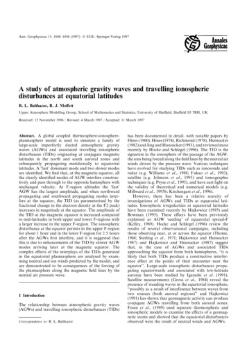
1052R. L. Balthazor, R. J. Mo ett: A study of atmospheric gravity waves and travelling ionospheric disturbancesFig. 6. Change in NmF2 (the density of the F2 peak), relative tosteady-state conditions, with only a northern auroral disturbance. Theformat of the plots is identical to that of Fig. 1Fig. 8. Vertical pro le of fractional change in electron concentrationat the magnetic equator at 162 E, from 12.15 UT to 19.50 UT.Contours are spaced every dNe 0:01. The solid (dotted ) lines arepositive (negative) contours. The broken line running left to rightacross the plot shows the height of the F2 peak, hmF2by the fast AGW, and in the Southern Hemisphereremains at lower altitudes as the slower waves passthrough.The signature of the TID clearly depends on theparameterisation used. Examining hmF2 (Fig. 4) showsa pattern that is both relatively symmetric latitudinallyabout the equator, and relatively stable in the spatialcorrespondence with the forcing AGW. In contrast, thechange in NmF2 (Fig. 5) is distinctly anti-symmetriclatitudinally about the equator, and has a very poorspatial correspondence to the forcing AGWs; this is alsoseen examining only a Northern-Hemisphere disturbance (Fig. 6), which shows the poor spatial correlationbetween the AGW and the TID.The vertical pro le of Ne at the magnetic equator isshown in Fig. 7. The lowering of the atmosphere duringthe night is clearly shown. The fractional change in Ne isshown in Fig. 8. The signature of the TID is approximately of equal magnitude both below and above theF2 peak. This may be contrasted with Fig. 9 showingpredictions for the wave passing through a low-latitudestation (24 N geographic), where the slow' southwardpropagating wave interferes with the fast' northwardpropagating wave (in a similar way to the two fast'waves interfering at the equator). The waves interfere at15.45 UT (02.33 LT). At this low latitude, the signatureof the TID is largest below the F2 peak, with thesignature in the upper F-region proportionally smaller.Figure 10 shows the equatorial data as a series ofindividual vertical pro les. At the equator, the verticalpro le initially exhibits a sharply peaked decrease in Necentred around 260 km (considerably below the F2peak) with an increase in Ne above 400 km. Thissituation then reverses between 15.15 and 15.30 UT(02.17 LT), when Ne increases rapidly below 350 km andFig. 7. Vertical pro le of electron concentration at the magneticequator at 162 E, from 12.15 UT to 17.00 UT. Values are Log10 Ne .Equally spaced contours are shown as solid lines, whilst dotted linesare intermediate arbitrary values chosen to show structure. Thecontours at 10.25 and 10.75 have been omitted for clarity. The fast'AGW passes over the magnetic equator between 14.45 and 16.00 UTFig. 9. Low latitude vertical pro le of fractional change in electronconcentration at 24 N (geographic), (16 N magnetic), 162 E (geographic), from 12.15 UT to 19.50 UT. Contours are spaced everydNe 0:025. The denotation of the contours and hmF2 are describedin Fig. 8
R. L. Balthazor, R. J. Mo ett: A study of atmospheric gravity waves and travelling ionospheric disturbances1053VaÈisaÈlaÈ period. Kelley (1989) gives sg at 380 km as lyingbetween 12 and 17 min; taking an approximation of15 min, we obtain kz 650 km at this altitude. This islarge compared with the thickness of the F2 peak, andso the passage of the AGW lifts the whole of the F2peak in phase; the change in sign of the fractionalchange in Ne thus simply corresponds to the change insign of the gradient of the F2 peak (after Thome, 1968).Figure 11 shows the same vertical pro le at the equatorover an extended time until 18.45 UT. The disturbanceis still present 5 h after the fast' waves interfere at theequator and decays slowly; the ions that were previouslytrapped at lower altitudes are now slowly moved back tothe upper F-region. Evidence can also be seen in Fig. 11of vertical wavelengths shorter than 650 km; it issuggested that these are harmonics of the wavelengthsassociated with both the fast' AGW and with thesubsequent slower' AGWs interfering.The e ect of the AGWs on the xed pressuresurfaces, the neutral winds and the ion winds are shownin Figs. 12, 13 and 14, giving cross-sections of theatmospheric wind patterns at 14.30 UT, 15.15 UT and16.15 UT respectively. As the two AGWs approach theequator at 14.30 UT (01.18 LT), the neutral atmosphereis lifted, pushing the ions up along the eld lines as inFig. 12. Here, the AGWs have a strong equatorwardwind caused by the pressure wave, driving the ions upFig. 10. Change in Ne at the magnetic equator from 100 to 600 km asthe AGWs pass overhead, on the line of geographic longitude 162 east. The solid lines show the fractional change in Ne from diurnallysteady-state conditions at successive times from 14.00 UT to 17.00UT. Each interval is 15 min, apart from the rst and last intervalswhich are 30 min. The dashed line in each plot shows fractionalchange in Ne at a point 10 north of the magnetic equator, whilst thedotted line shows the fractional change in Ne 10 south of themagnetic equatordecreases above that altitude. At ten degrees north andsouth of the magnetic equator, the vertical pro le issimilar, but the fractional changes in Ne at around260 km are considerably larger than at the equator; thisis a consequence of the larger dip angle of the magnetic eld at mid-latitudes, where the mainly horizontalforcing neutral winds may drive the ions with a largervertical component of motion. The explanation of thereversal of the sign of the fractional change in Ne may befound by examining the vertical wavelength of theforcing AGW. From the standard analysis of atmospheric wave propagation (Hines, 1960), rearrangingterms and taking the approximation x xa (theacoustic wave frequency), the dispersion relation maybe written as!s2g2kz 21 k2s ÿ s2g xwhere kx is the horizontal wavelength, kz is the verticalwavelength, s is the wave period and sg is the Brunt-Fig. 11. Change in Ne at the magnetic equator from 100 to 600 km asthe AGWs pass overhead, on the line of geographic longitude 162 east. The vertical pro les show the fractional change in Ne at themagnetic equator every 15 min from 14.00 UT to 18.45 UT
1054R. L. Balthazor, R. J. Mo ett: A study of atmospheric gravity waves and travelling ionospheric disturbancesFig. 12. A slice through the atmosphere at a xed longitude on thegeographic meridian 162 E, from 10 S to 25 N and from 100 km to450 km in altitude, at UT 14.30. The upper plot shows a schematic ofthe main behaviour of the plot, and is not to scale. Shaded areas showregions where the height of xed pressure levels is increased due to thepassage of the AGW, whilst solid (hollow) arrows show changes in theneutral (ion) winds. The contour plot below (with arbitrary levels ofcontours chosen to illustrate the structure) shows the fractionalchange (from diurnal steady-state conditions) of the height of thethermospheric xed pressure levels, due to the passage of the AGWs.The thick solid arrows show the direction and comparative magnitudeof the change in the component of the neutral wind in this meridian.The looped dotted lines show the projections of the nearest calculatedadjacent ux tubes onto the geographic meridian. The thin openarrows show the direction and magnitude of the change in the ionwind due to this uctuation from steady state conditions. Althoughthe size of each arrow is proportional to the magnitude of the windcomponent, the magnitude of the ion wind arrows has been multipliedby a factor of 10 to show more clearly the direction of the (smaller)ion windthe eld lines. The horizontal wind increases withaltitude (corresponding to the decrease in pressure).The sloping phase front of the AGW is evident below250 km, indicating an upward ow of energy.At 15.15 UT (02.03 LT), the two AGWs havecombined over the magnetic equator. Above 250 km,the pressure gradient is now driving a horizontal neutralwind polewards into each hemisphere, forcing the ionsback down the ux tubes (and enhancing the equatorialanomaly in each hemisphere). Below 250 km there isinterference between the slower and faster AGWs,Fig. 13. As Fig. 12, except the slice is taken at 15.15 UT. The upperpanel shows the main features of the plot. The contour levels (lowerpanel ) are identical to Fig. 12resulting in smaller pressure gradients. The neutralwinds are reduced and there are residual ion motionsfrom the previous timestep.At 16.15 UT (03.03 LT), the two fast AGWs havenow passed into the opposing hemispheres. Above250 km, each wave is now distinct, the pressure gradientsforcing the neutral atmosphere meridionally away fromeach wave, and the trailing edges of the AGWs are seen.Ions in the upper sections of the ux tubes areconsequently driven upwards once again (although it isnoted that there is a net neutral wind southward acrossthe magnetic equator, forcing ions over the top of the ux tubes). In the region above about 180 km but below250 km, the slow AGWs are interfering and resulting ina pressure gradient away from the magnetic equator,forcing a poleward neutral wind into each hemisphere.4 Concluding remarksThe global fully coupled thermosphere ionosphere plasmasphere model has been used to simulate AGWsoriginating from an electric- eld enhancement at auroral latitudes, and propagating to equatorial latitudes,along with the associated TID signatures. The AGWs
R. L. Balthazor, R. J. Mo ett: A study of atmospheric gravity waves and travelling ionospheric disturbances1055above the F2 peak decays over a period of about 1 h,whilst the perturbation below the F2 peak decays moreslowly over a period of several hours. It is suggested thatthe persistence of the lower F-region disturbance is dueto the arrival at the equator of pairs of slower AGWsgenerated by the original auroral source, which act tocounter the decaying perturbation caused by the rst fast' pair of AGWs. We also note this study hassimulated a single impulsive event which generated afamily of single large-scale gravity waves. Studies by e.g.Williams et al. (1988) have shown that there can be aperiodicity to the source mechanism to produce anAGW wave-train, and such a wave-train could furtherprolong the decay of the lower F-region equatorialdisturbance as suggested by Gross et al. (1984).Acknowledgements. This work has been supported by the UKScience and Engineering Research Council and Particle Physicsand Astronomy Research Council.Topical Editor D. Alcayde thanks H. Hocke and R. V. Lewisfor their help in evaluating this paper.ReferencesFig. 14. As Fig. 12, except the slice is taken at 16.15 UT. The upperpanel shows the main features of the plot. The contour levels (lowerpanel ) are identical to Fig. 12are identi ed as a family of imperfectly ducted wavemodes. The fundamental mode of this family have beenpredicted by simple thermospheric models e.g. Francis,(1973) and the more complex coupled model used herepredicts additional slower modes of smaller amplitude.These are in agreement with observations by Thome(1968) and Hajkowicz and Hunsucker (1987).The behaviour of the AGWs and TIDs at the equatorhas been studied in detail and the complex observablecharacteristics of the TIDs are explained by the behaviour of the forcing horizontal neutral winds. Observingthe ionosphere only at one height (e.g. NmF2 or hmF2)presents an incomplete picture of the family of TIDs.The conjugate AGWs originating in both north andsouth auroral zones interfere constructively at theequator and the magnitude of the TID is slightlyincreased, con rming the suggestion of Hajkowicz andHunsucker (1987) and the statistical survey ofHajkowicz (1991). The TIDs
AGWs and TIDs at equatorial latitudes will henceforth ignore the initially poleward-travelling waves, and refer to the equatorially-travelling waves as 'northward-trav-elling' (originating in the Southern Hemisphere) and 'southward-travelling' (originating in the Northern Hemisphere) respectively. The waves interfere at the