Transcription
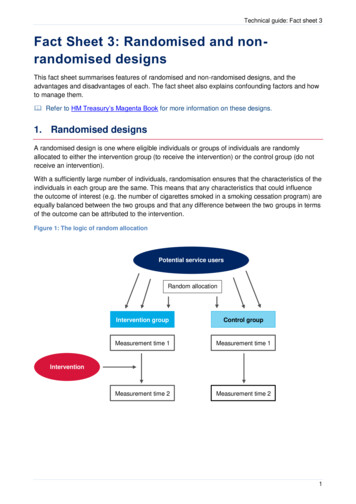
Technical guide: Fact sheet 3Fact Sheet 3: Randomised and nonrandomised designsThis fact sheet summarises features of randomised and non-randomised designs, and theadvantages and disadvantages of each. The fact sheet also explains confounding factors and howto manage them. Refer to HM Treasury’s Magenta Book for more information on these designs.1. Randomised designsA randomised design is one where eligible individuals or groups of individuals are randomlyallocated to either the intervention group (to receive the intervention) or the control group (do notreceive an intervention).With a sufficiently large number of individuals, randomisation ensures that the characteristics of theindividuals in each group are the same. This means that any characteristics that could influencethe outcome of interest (e.g. the number of cigarettes smoked in a smoking cessation program) areequally balanced between the two groups and that any difference between the two groups in termsof the outcome can be attributed to the intervention.Figure 1: The logic of random allocationPotential service usersRandom allocationIntervention groupControl groupMeasurement time 1Measurement time 1Measurement time 2Measurement time 2Intervention1
Technical guide: Fact sheet 31.1 Individual randomised designAn individual randomised design randomly allocates eligible individuals to either the interventiongroup or the control group. Typically, in a randomised design with two groups (one intervention andone control), there is a 50:50 chance of eligible individuals being allocated to either group.Box 1: Example of individual randomised designLet us consider a new rehabilitation program aimed at reducing recidivism following release fromcustody. At the time of release, eligible individuals could be randomly allocated to therehabilitation program (intervention group) or standard practice (control group).1.2 Cluster randomised designWhen randomisation of individuals is not practical or desirable, you could consider clusterrandomised designs where groups (or “clusters”) of individuals are randomly allocated to either theintervention or control group. This is often the case when an intervention is better delivered togroups of individuals (e.g. group training sessions or geographical rollout). Cluster trials also helpprevent “contamination bias” where individuals receiving the intervention influence those notreceiving the intervention when in close proximity.Box 2: Example of cluster randomised designLet us consider an intervention that aims to prevent harassment and bullying in primary schoolchildren via face-to-face training sessions. In this instance, it would be difficult to randomiseindividuals from the same school to either the intervention or control group for two reasons:1. Children from the same school are likely to talk to each other and share the informationlearned during the training sessions with those randomly allocated to the control group(“contamination” bias).2. It seems more natural and effective for such an intervention to be delivered at the school level.Using a cluster randomised design, you could select all schools within a geographical area (e.g.Sydney) and randomly allocate schools to either receive or not receive the intervention.1.3 Stepped-wedge designOne disadvantage of traditional randomised designs, both with individual and clusterrandomisations, is that (typically) half of the eligible population is allocated to a control group anddoes not receive the intervention. While this is acceptable when there is clear uncertainty about thepotential benefits of an intervention (e.g. a new drug in a drug trial), it can pose ethical andlogistical problems when the intervention is strongly believed to have benefits which are difficult towithhold from eligible individuals. In this instance, alternative randomised designs involving adelayed intervention can be considered. Those designs are generally called “stepped-wedge”designs and involve randomly allocating individuals or groups of individuals to different startingtimes.11Hemming K., & Taljaard M. (2015) Sample size calculations for stepped wedge and cluster randomisedtrials: a unified approach. Journal of Clinical Epidemiology. 69:137-146.2
Technical guide: Fact sheet 3For example, with three randomly allocated groups, one group would start the intervention straightaway, the second group a bit later, and the third group even later. With this design, everyone whois eligible receives the intervention while maintaining the advantages conferred by randomisation(i.e. making sure that all three groups are comparable).Box 3: Example of stepped-wedge designLet us consider again the school bullying example. There may be some who consider theintervention should be offered to all schools or perhaps some schools are reluctant to participate.In these cases, you could consider a stepped-wedge design where schools are randomlyallocated to different starting dates. A possible stepped-wedge design could involve three groupsof schools starting the intervention at three different times. All end up receiving the training.The design is represented in the table below where dark blue cells represent the period/s whenschools are receiving the intervention. In the first period, none of the schools receive theintervention, providing baseline information on the rate of bullying and harassment in the absenceof an intervention. At each subsequent period, the intervention is introduced to a new group ofschools. By the fourth period, all schools are receiving the intervention.Period 1Period 2Period 3Period 41st groupof schools2nd groupof schools3rd groupof schools2. Non-randomised designsRandomised designs may not always be appropriate or feasible. This may be the case whenimplementing macro policies or system-wide changes where it is difficult to influence interventionallocation or when it may be seen as unethical to withhold an intervention already proven to beeffective. Under those circumstances, it is still essential to have an appropriate control group whichwill be observed and measured as similarly as possible as the intervention group.The main drawback of non-randomised designs is the limited ability to guarantee the comparabilityof the intervention and control groups. Proposals to use a non-randomised control group should, asmuch as possible, adhere to the following rules (note that points 3 and 4 also apply to randomiseddesigns):1.Collect baseline data on all known confounds (i.e. characteristics with the potential toinfluence the outcomes) for both the intervention and control groups.2.Collect data on the primary outcome at multiple times in both groups, with at least one datapoint before the start of the intervention and at least one after. This is so you can try toseparate the effect of the intervention from other factors in the environment.3.Ensure that both the intervention and control groups are observed at the same time.4.Ensure that both the intervention and control groups follow the same data collectionprocedure.3
Technical guide: Fact sheet 3However, sophisticated non-randomised designs are available to help strengthen basic controlledbefore-and-after approaches, especially where confounds are well understood and measured,causal pathways to outcomes are known, and the impact is anticipated to be large.Assuming the above rules can be followed, a range of methods is then available for establishingthe counterfactual. The main ones involve: multivariable analyses matching (e.g. using propensity scoring) comparing changes over time between the intervention and control groups (sometimes called“difference in differences”).In most cases, analysis involves a mixture of the above methods. For example, by first identifying awell-matched subset of individuals using a propensity score and then by comparing changes overtime between the intervention and control groups. More details about these methods are availablein Sections 9.33 to 9.48 of the Magenta Book.2.1 Non-randomised designs with a control groupPropensity score matchingPropensity scoring calculates the probability of being a participant in an intervention given a rangeof individual characteristics measured before enrolling in the intervention, both for interventionparticipants and individuals not participating. This is typically done using a logistic regressionwhere the outcome is an indicator of enrolment (yes or no) and predictors include a range offactors with the potential to influence enrolment and/or outcomes. Once the probability has beencalculated for everyone, the idea is to match each intervention participant to one or more controlparticipants with the same probability. Those with no appropriate match are not included in theanalysis and individual characteristics across the two groups are balanced.The main limitation of propensity matching is that, as opposed to randomisation, it is only able tobalance observed characteristics. For more details, refer to Peter Austin’s introduction topropensity score methods.2Box 4: Example of propensity score matching – UK’s Peterborough social impactbond (SIB)3The Peterborough SIB aimed to reduce reconviction rates for short sentence male prisonersleaving HMP Peterborough. It was launched in September 2010 and provided interventions foradult males (aged 18 years or over) receiving custodial sentences of less than 12 months (‘shortsentence prisoners’) and discharged from HMP Peterborough.The UK Ministry of Justice and Social Finance proposed a matched control group to remove theinfluence of external events on reconviction levels (e.g. changes in sentencing policy, theeconomic environment, etc.). Consequently, the approach outlined in the SIB contract was todevelop a control group of prisoners discharged from other prisons during the same time period asthe Peterborough cohort. This control group was developed using propensity score matching.2Austin P. (2011) An introduction to propensity score methods for reducing the effects of confounding inobservational studies. Multivariate Behav Res.; 46(3): 399-4243Cave, Williams, Jolliffe & Hedderman (2012); Jolliffe & Hedderman (2014)4
Technical guide: Fact sheet 3The 936 men released from HMP Peterborough and 9,360 released from other prisons weresuccessfully matched on the propensity score in terms of demographics and criminal history. Theanalysis showed an 8.39% reduction in reoffending rates within the Peterborough Cohort 1, whichwas greater than the control group but insufficient to trigger payment under the terms of the bond.Difference-in-difference designDifference-in-difference designs use time trends in an outcome. In this design, trends in associatedoutcomes between intervention and control groups are compared over a time period relevant to theintervention. While unobserved factors might affect the outcome, if they do not affect trends in theoutcome, then the trends for both groups in the absence of the intervention will be the same. Anysignificant difference in trends can be interpreted as an intervention effect. This is the so-calledparallelism or “common trends” assumption.The parallelism assumption should always be verified where possible, either by examining the preintervention trends in historical time series data or from previous studies. Where the assumptiondoes hold, this design is a useful method that can address selection bias in the absence of richinformation about the participants. But the parallelism assumption should not be automaticallyassumed true, and this approach would not be recommended if, for example, data are onlyavailable at two time points (before and after the implementation of an intervention). The basicapproach of this design to consider an intervention reconfiguration is illustrated below. 4Figure 2: Difference-in-difference design4Morris, S. et al. (2014). Impact of centralising acute stroke services in English metropolitan areas onmortality and length of hospital stay: difference-in-differences analysis. BMJ, 349, g47575
Technical guide: Fact sheet 3Box 5: An example of a difference-in-difference evaluation5WHC ran a pilot from February 2006 to February 2008. It was a free, no-obligation service thataimed to provide small and medium-sized enterprises with advice on workplace health issues toincrease the level of healthy workplaces across England and Wales.The primary outcome of interest was a net beneficial impact on the incidence and duration ofoccupationally related ill-health and injury. Employers operating in regions where the WHCworkplace visit service was not provided were the control group, on the basis that they were similar(in terms of their size and sector) to those participating in the WHC pilot. Their outcomes,therefore, constituted the best available estimate of the counterfactual.One way of evaluating the impact of the WHC pilot would have been to look directly at therelationship between involvement in the pilot and final outcomes. However, this approach wasconsidered unlikely to produce robust results because, in addition to improving safety, using thepilot can change the way final outcomes are recorded.Instead the relationship was analysed in two stages, looking first at the effect of the WHC pilot onintermediate outcomes and then looking at the effect of the intermediate outcomes on the finaloutcomes. These relationships were examined using difference-in-difference analysis. This lookedat the changes in outcomes between the two survey waves, and tested whether these changeswere different for the WHC pilot intervention and control groups. There was no evidence that takingpart in WHC had a direct measurable effect on absenteeism due to illness. There was, however,evidence that involvement in WHC improved a range of health and safety practices. These werelinked to reduced accident rates.5For more guidance, see HM Treasury (2011), The Magenta Book. Guidance for evaluation6
Technical guide: Fact sheet 3Replicated interrupted time seriesAn extension of the simple difference-in-difference design consists of taking one or moreobservations from both the intervention and control groups prior to introducing an intervention. Thisis sometimes called an ‘interrupted time series’. If the intervention is working, we would expect thesecond set of observations to move in a more favourable direction for the intervention group thanfor the control group. Notice that by comparing outcomes for both intervention and control groupsafter the intervention, we are able to control for any known factors that might be influencing trendsin both groups. An example of this design is provided in the figure below.Figure 2: Hypothetical example of a replicated interrupted time series design2.2 Non-randomised designs without a control groupSimpler comparisons can be illuminating, but can be difficult to interpret because they do notinclude a way to estimate the counterfactual. These methods6 include for example: comparing before and after the intervention comparing ‘dose’ of change or degree of exposure to change across settings regression discontinuity design instrumental variable estimation.In general, designs with no control group are discouraged as they do not provide a reliableopportunity to separate the effect of an intervention from possible simultaneous changes occurringover the course of the program. However, it is recognised that in exceptional circumstances suchdesigns may be justifiably proposed.6For more guidance, see HM Treasury (2011), The Magenta Book. Guidance for evaluation7
Technical guide: Fact sheet 33. SummaryIn summary, a randomised trial provides the most reliable framework for assessing the impact ofan intervention because, when sufficiently large it provides a control group that only differs from theintervention group in terms of the intervention being received or not. Table 1 below brieflysummarises the advantages and disadvantages of each design.Table 1: Advantages and disadvantages of main vidual trialBalances both measured andunmeasured confounds.Can be resource intensive and/or notacceptable for certain interventions.Provides the most robust evidence ofimpact.Those randomised out of the interventionwill not be able to receive the intervention.Randomisedcluster trialAbility to randomise clusters/groups ofindividuals when individual randomisationis not appropriate.Increases the sample size compared toan individual randomised trial.Stepped-wedgetrialAllows everyone to receive theintervention while retaining the benefits ofrandomisation.Takes longer than an individual or clustertrial and is more complex to analyse.Propensitymatched controlProvides a more flexible framework than arandomised design with a plausiblecounterfactual.Substantially increases the risk of bias inthe presence of unmeasured confounds.Difference-indifferenceProvides a more flexible framework than arandomised design with a plausiblecounterfactual.Substantially increases the risk of bias inthe presence of unmeasured confounds.Interrupted timeseriesMore flexible than randomisation, makinguse of time trends and a plausiblecounterfactual.Difficult to attribute effect to theintervention due to the absence of acounterfactual; can be strengthened byaddition of an observed control group.8
advantages and disadvantages of each. The fact sheet also explains confounding factors and how to manage them. Refer to HM Treasury's Magenta Book for more information on these designs. 1. Randomised designs A randomised design is one where eligible individuals or groups of individuals are randomly