Transcription
ASPHERIC ORIENTATIONS OF SIMPLICIAL COMPLEXESA thesis presented to the faculty ofSan Francisco State UniversityIn partial fulfillment ofThe requirements forThe degreeMaster of ArtsInMathematicsbyLogan GodkinSan Francisco, CaliforniaJune 2012
Copyright byLogan Godkin2012
CERTIFICATION OF APPROVALI certify that I have read ASPHERIC ORIENTATIONS OF SIMPLICIAL COMPLEXES by Logan Godkin and that in my opinion this workmeets the criteria for approving a thesis submitted in partial fulfillmentof the requirements for the degree: Master of Arts in Mathematics atSan Francisco State University.Matthias BeckProfessor of MathematicsFelix BreuerProfessor of MathematicsJeremy MartinAssociate Professor of MathematicsUniversity of Kansas
ASPHERIC ORIENTATIONS OF SIMPLICIAL COMPLEXESLogan GodkinSan Francisco State University2012We generalize the notions of colorings, flows, and tensions of graphs to simplicialcomplexes, and then to cell complexes, by viewing a graph as a one dimensionalsimplicial complex. We look at both integral and modular colorings, flows, andtensions of cell complexes. The functions that count colorings, flows, and tensionsfor graphs are known to be polynomials. We show that these counting functions forcell complexes are in general quasipolnomials and for the modular counting functionswe give sufficent conditions for these functions to be polynomials. Furthermore, weshow that these modular counting functions are evaluations of the Tutte polynomial.We show that for certain cell complexes we can generalize the deletion-contractionoperation for graphs and use it to compute these modular counting functions. Wegeneralize the reciprocity results for these integral counting fucntions of graphs tocell complexes via inside-out polytopes and Ehrhart–Macdonald reciprocity.I certify that the Abstract is a correct representation of the content of this thesis.Chair, Thesis CommitteeDate
ACKNOWLEDGMENTSI thank my advisor, Dr. Matthias Beck, for his help and all the oppurtunities he gave me for without them I would be much worse off. I thankDrs. Felix Breuer and Jeremy Martin whose help has advanced my mindgreatly and whose ideas are integral to this thesis.Finally, I thank my parents, John and Patricia Godkin, for being thebest parents anyone can hope for and for supporting me in everything Ido. I dedicate this thesis to them.v
TABLE OF CONTENTS1 Introduction . . . . . . . . . . . . . . . . . . . . . . . . . . . . . . . . . . .11.1Motivation . . . . . . . . . . . . . . . . . . . . . . . . . . . . . . . . .11.2Simplicial Complexes . . . . . . . . . . . . . . . . . . . . . . . . . . .31.3Homology . . . . . . . . . . . . . . . . . . . . . . . . . . . . . . . . .72 Deletion-Contraction and Inclusion-Exclusion . . . . . . . . . . . . . . . . 112.12.2The Modular Coloring Function . . . . . . . . . . . . . . . . . . . . . 142.1.1Deletion-Contraction Examples . . . . . . . . . . . . . . . . . 192.1.2Inclusion-Exclusion Examples . . . . . . . . . . . . . . . . . . 30The Modular Tension Function . . . . . . . . . . . . . . . . . . . . . 312.2.12.3A Modular Tension Example . . . . . . . . . . . . . . . . . . . 36The Modular Flow Function . . . . . . . . . . . . . . . . . . . . . . . 363 Integral Counting Functions and their Reciprocity . . . . . . . . . . . . . . 423.1k-Colorings and Aspheric Orientations . . . . . . . . . . . . . . . . . 423.1.1A k-coloring Example. . . . . . . . . . . . . . . . . . . . . . 483.2k-Tensions and Aspheric Orientations . . . . . . . . . . . . . . . . . . 493.3k-Flows and Totally Spheric Orientations . . . . . . . . . . . . . . . . 52Bibliography . . . . . . . . . . . . . . . . . . . . . . . . . . . . . . . . . . . . 56vi
Chapter 1Introduction1.1 MotivationIn this section we give some motivation for how we define colorings, tensions, andflows for cell complexes. These definitions are based on the boundary matrix of acell complex and since we wish to extend ideas from graph theory to cell complexeswe start by constructing the boundary matrix of a graph.Let G (V, E) be a graph with vertex set V and edge set E. Let e vu be anedge of G, where v and u are the vertices incident to e. Then we can give the edgee an orientation by writing its vertices as an ordered pair e (v, u). We say thate is directed from v to u, and we say that v is the tail and u is the head. Givingan orientation to each edge of G we obtain an oriented graph G0 . We construct theboundary matrix B of G0 , a V E -matrix whose rows are indexed by the vertices1
2of G0 and whose columns are indexed by the edges of G0 , by setting the ve-entryequal to 1 if v is the tail of e; 1 if v is the head of e; 0 otherwise (see [4] for more).Now let G be an oriented graph. A path of G is a sequence of vertices {v1 , . . . , vn }such that v1 v2 , v2 v3 , . . . , vn 1 vn are edges of the graph and the vi are all distinct. Acycle C of a graph is a closed path, that is, if the sequence {v1 , v2 , . . . , vn } representsa cycle of G, then the cycle has edges v1 v2 , v2 v3 , . . . , vn 1 vn , vn v1 . If G is an orientedgraph, then an oriented cycle C of G is a sequence of vertices {v1 , v2 , . . . , vn } suchthat (v1 , v2 ), (v2 , v3 ), . . . , (vn 1 , vn ), (vn , v1 ) are oriented edges of G. It can be shownthat any cycle C of G can be represented as an element s in { 1, 0, 1}E such thatBs 0 and, vice versa, any element s in { 1, 0, 1}E such that Bs 0 representsa cycle C of G. Furthermore, any oriented cycle C of G can be represented as anelement s in {0, 1}E such that Bs 0 and, vice versa, any element s in {0, 1}Esuch that Bs 0 represents an oriented cycle C of G. It can be shown that theset of cycle vectors of a graph form a basis for the null space (over R) of B (see [4]and [5, Chapter 14.2] for more).An A-coloring of G is a labeling of the vertices of G with elements of A, whereA is a commutative ring with unity. A proper A-coloring of a graph is a labelingof the vertices such that there do not exist adjacent vertices labeled by the sameelement of A. We can think of an A-coloring as an element c in AV . Thus c is aproper A-coloring if cB is nowhere-zero.An A-tension of G is a labeling of the edges of G with elements of A such that
3each oriented sum of edge labelings on each cycle of G is zero. We say that anA-tension is nowhere-zero if none of the edge labels are zero. We can represent anA-tension as an element ψ in AE such that ψ · s 0 for every cycle s of G, and ψis nowhere-zero if none of the entries of ψ are zero.An A-flow of G is a labeling of the edges of G with elements of A such that theoriented sum of edge labelings at each vertex is equal to zero, that is, the sum ofthe edge labelings whose edges are directed to the vertex v equals the edge labelingswhose edges are directed away from v. We say that an A-flow is nowhere-zero ifnone of the edge labels are zero. We can represent an A-flow as an element φ in AEsuch that Bφ 0, and φ is nowhere-zero if none of the entries of φ are zero.An oriented graph G is said to be acyclic if G does not contain any orientedcycles or equivalently if the null space of B (over R) does not contain any nonzerovector in {0, 1}E . We say that G is totally cyclic if every edge of G belongs to someoriented cycle or equivalently if for every edge e there is a vector in {0, 1}E in thenull space of B whose e-entry is nonzero.1.2 Simplicial ComplexesIn this section we will construct the bounday matrix of a simplicial complex. Wewill use the boundary matrix of a simplicial complex to define colorings, tensions,and flows of cell complexes as we did for graphs in the previous section.A simplicial complex X is a collection of finite nonempty sets (the faces of X)
4such that if Y is an element of X, then so is every nonempty subset of Y . An elementof cardinality d 1 is called a d-dimensional simplex or more simply d-simplex.We say X is d-dimensional if the maximum cardinality of any element of X is d 1.For any d-dimensional simplicial complex X, let F denote the set of d-dimensionalsimplices called facets, let R denote the set of (d 1)-dimensional simplices calledridges, and let V denote the 0-dimensional simplices called vertices (see [6] formore on simplicial complexes).The boundary matrix, denoted [ d ], of a d-dimensional simplical complex Xis an R F -matrix where the rows are indexed by the ridges and the columnsare indexed by the facets of X. The entries of [ d ] are obtained from the followingsetup.1. Fix a total ordering of the vertices of X. Given that V k, we fix a totalordering via a bijection V [k], where [k] : {1, 2, . . . , k}.2. Orient each face of X by writing its vertices in an increasing order, thatis, a d-face D with vertex set {v0 , v1 , . . . , vd } will produce a chain [D] [v0 , v1 , . . . , vd ]. The chain group, denoted Cd (X), is the free Z-module ofZ-linear combinations of d-dimensional simplices, represented by their chains.3. Define the d-th boundary map (see, for instance, [6]) d : Cd (X) Cd 1 (X)bydX d ([v0 , v1 , . . . , vd ]) ( 1)j [v0 , ., vj 1 , vj 1 , ., vd ].j 0
5If f [v0 , v1 , . . . , vd ] is a facet of X and r [v0 , ., vj 1 , vj 1 , ., vd ] is a ridgeof f , then the rf -entry in [ d ] is ( 1)j and otherwise 0.Remark. From the construction of the boundary matrix of a simplicial complex weget that the nonzero entries in each column must alternate in sign. Thus, since thereare two possibilities for how the nonzero entires alternate in sign, we see that eachfacet of a simplicial complex can have two orientations. Hence a reorientation of afacet can be given by multiplying the appropriate column of the boundary matrixby 1.Let X be a simplicial complex with boundary matrix [ ]. We define a boundarymatrix orientation of X to be an element o of { 1, 1}F . We reorient X by scalarmultiplying every column fi of the boundary matrix [ ] of X by the correspondingentry oi in the orientation vector o. Note that the initial boundary matrix has theorientation o in {1}F .We call the vectors belonging to the null space (over R) of [ d ] the cycles of Xand from now on we will refer to this null space as the cycle space. We define asphere (simple cycle) of X to be an element s of ZF belonging to the cycle spaceof [ d ] and an oriented sphere (oriented cycle) of X to be an element s of NFbelonging to the cycle space of [ d ], where N is the set of nonnegative integers. Asimplicial complex X is aspheric (acyclic) if there does not exist a nonzero elements of NF in the cycle space of [ d ] and we say X is totally spheric (totally cyclic)if for every facet fi of X we have an element s of NF with a nonzero ith-entry in
6the cycle space of [ d ].An A-coloring of X is an element c of AR , where A is a commutative ring withunity, and we say the coloring is proper if c·[ d ] is nowhere-zero in A. A k-coloring(integral coloring) of X is a coloring that is an element of [ k, k]R , where A Zand [ k, k] : { k, . . . , 1, 0, 1, . . . , k}. A Zk -coloring (modular coloring) of Xis a coloring, where A Zk .Note. As far as we know, the concept of proper colorings has not been studied forsimplicial complexes.An element φ of AF is an A-flow if [ d ] · φ 0 in A. Thus, the null space (overA) of [ d ] contains all of the flow vectors of a simplicial complex. A k-flow of X isa nonzero element φ of [ k, k]F that is a flow in Z, and a Zk -flow of X is a nonzeroelement φ of ZFk that is a flow in Zk . We define the flow space of X to be the nullspace of [ d ] over A.An A-tension is an element ψ of AF such that ψ · q 0 in A for every vectorq in the cycle space of [ d ]. Thus every A-linear combination of row vectors from[ d ] is an A-tension. A k-tension of X is a nonzero element ψ of [ k, k]F suchthat ψ · q 0 in Z and a Zk -tension of X is a nonzero element ψ of ZF such thatψ · q 0 in Zk , for every vector q in the cycle space of [ d ].We define the order of a simplicial complex X to be the number of ridges in X,and the degree of a ridge is the number of facets that have the ridge as a boundary.Proposition 1.1. In a simplicial complex X, the sum of degrees of the ridges is
7equal to (d 1) times the number of facets, where d is the dimension of X.Proof. LetS Xdeg(r)r Rand let the dimension of X be d. Note that we count each facet exactly d 1 times.Thus, S (d 1) F .Corollary 1.2. Let X be a d-dimensional simplicial complex. If d is odd, then thenumber of ridges with odd degree is even, and if d is even, then the number of ridgeswith odd degree is odd if F is odd and even if F is even.1.3 HomologyWe begin with an introduction to homology (taken from [6]), and then proceed togive a construction of cell complexes and their corresponding boundary matrices.We start with a sequence of homomorphism of abelian groups n 1 n10· · · Cn 1 Cn Cn 1 · · · C1 C0 0where n n 1 0 for each n and 0 0. We refer to such a sequence as a chaincomplex. It follows that the image of n 1 , denoted Im , is a subset of the kernelof n , denoted ker n . Then the n-th homology group of the chain complex is thequotient group Hn ker n / Im n 1 .
8When X is a simplicial complex the Ci are groups whose elements are Z-linearcombinations of i-dimensional faces (as described in Section 1.2).We define the reduced homology group H̃n (X) to be the homology groupsof the augmented chain complex ε21· · · C2 (X) C1 (X) C0 (X) Z 0PPwhere ε ( i ni σi ) i ni , σi is a chain in C0 , and ni is an integer.Given a space X and a subspace Y X, let Cn (X, Y ) be the quotient groupCn (X)/Cn (Y ). Since the boundary map : Cn (X) Cn 1 (X) takes Cn (Y ) toCn 1 (Y ) we have the induced quotient boundary map : Cn (X, Y ) Cn 1 (X, Y ).Then we have a chain complex n 1 10· · · Cn 1 (X, Y ) Cn (X, Y ) · · · C1 (X, Y ) C0 (X, Y ) 0.The relative homology group Hn (X, Y ) is ker n / Im n 1 .An n-cell en is an open n-dimensional ball (up to homeomorphism). We construct a cell complex X in the following way using the construction from [6]:1. Start with a finite set of 0-cells denoted X 0 .2. Inductively, form the n-skeleton X n from X n 1 by attaching n-cells eni viamaps αi : S n 1 X n 1 . This means that X n is the quotient space of the
9disjoint union X n 1Din of X n 1 with a collection of n-disks Din under the identifications x αi (x) for x Din . As a set, X n X n 1 i eni . i3. We stop at some finite n and set X X n .We say a cell complex X is n-dimensional if X X n . Given an n-dimensionalcell complex we will refer to the n-cells as facets and the (n 1)-cells as ridges.Given a map f : S n S n , the induced map f : H̃n (S n ) H̃n (S n ) is ahomomorphism of the form f (x) αx, where α is some integer that depends onlyon f [6]. This integer α is called the degree of f [6].The cellular boundary formula is given [6] by dn (enf ) Prdrf ern 1 where drfis the degree of the mapSfn 1 Df X n 1 X n 1 Srn 1 ,X n 1 ern 1that is, the composition of the attaching maps of enf with the quotient map collapseX n 1 \ en 1to a point [6].rWe form the n-th boundary matrix [dn ] of a cell complex X by indexing therows by the ridges and the columns by the facets of X. We set the rf -entry in [dn ]to drf , where drf is given by the cellular boundary formula.Remark. A boundary matrix of a cell complex is an integer matrix since the drfentry in [dn ] is always an integer and any integer matrix is the boundary matrixof some cell complex since we can construct a cell complex where the en cell f is
10wrapped around the boundary of the en 1 cell r any integer number of times.Since our definitions in section 1.2 only depend on the boundary matrix of oursimplicial complex we will extend those definitions by replacing the “boundary matrix of a simplicial complex” with that of the “boundary matrix of a cell complex”.Proposition 1.3. Let X be a d-dimensional cell complex. We have a proper Acoloring c if and only if we have a nowhere-zero A-tension ψ, where ψ is an A-linearcombination of row vectors of [ d ].Proof. Assume c is a proper A-coloring. Then c[ d ] ψ is nowhere-zero and sinceψ is an A-linear combination of row vectors of [ d ] we have that ψ · q 0, where q isany cycle. Assume ψ is an A-tension that is an A-linear combination of row vectorsof [ d ], that is,Xcr br ψ,r Rwhere br is a row of [ d ] and cr A for all r R. Thus c (cr )r R is a propercoloring of X since ψ is nowhere-zero.
Chapter 2Deletion-Contraction andInclusion-ExclusionWe define deletion and contraction of a facet of a cell complex in terms of operationson the boundary matrix and note that the contraction operation is not alwayspossible.We define the deletion of a facet f of a cell complex X to be the cell complexX without the facet f . In terms of the boundary matrix [ n ] of X n X, the deletionof the facet f corresponds to the removal of the column in [ n ] corresponding to thefacet f . We denote the cell complex obtained from the deletion of f by X \ f .We define the contraction of a facet f of a cell complex X to be the followingpivot operation on the boundary matrix of X, where the pivot operation of amatrix B selects a nonzero entry brf , a pivot, in B and performs the following11
12steps: 1. For each row i 6 r of B, replace row i by row i 2. Multiply row r bybifbrf row r,1.brfRemark. The contraction of a facet f of a cell complex is, in general, not uniquesince we may any ridge r of f .Remark. It is possible that the contraction of a facet f of a cell complex does notresult in an integer matrix. For our purposes we restrict our choices of pivot elementsto 1 entries in our boundary matrix.A matrix is totally unimodular if and only if the determinant of each squaresub-matrix is 1, 0, or 1. We have the following theorems from [3]:Let X be a compact Hausdorff space. A curved triangle in X is a subspaceA of X and a homeomorphism h : T A, where T is a closed triangular regionin the plane. If e is an edge of T , then h(e) is said to be an edge of A; if v isa vertex of T , then h(v) is said to be a vertex of A. A triangulation of X is acollection of curved triangles A1 , . . . , An in X whose union is X such that for i 6 j,the intersection Ai Aj is either empty, or a vertex of both Ai and Aj , or an edgeof both. Furthermore, if hi : Ti Ai is the homeomorphism associated with Ai , werequire that when Ai Aj is an edge e of both, then the map h 1j hi defines a linear 1homeomorphism of the edge h 1i (e) of Ti with the edge hj (e) of Tj [7].An n-dimensional manifold is a Hausdorff space M such that each point hasan open neighborhood homeomorphic to Rn . A local orientation of M at a point
13x is a choice of generator µx of the infinite cyclic group Hn (M, M {x}). Anorientation of an n-dimensional manifold M is a function x 7 µx assigning toeach x M a local orientation µx Hn (M, M {x}), satisfying the condition thateach x M has a neighborhood Rn M containing an open ball B of finite radiusabout x such that all the local orientations µy at points y B are the images ofone generator µB of Hn (M, M {x}) Hn (Rn , Rn B) under the natural mapsHn (M, M B) Hn (M, M {y}). If an orientation exists for M , then M is calledorientable [6].Theorem 2.1. [3, Theorem 4.1] For a finite simplicial complex X triangulating a(d 1)-dimensional compact orientable manifold, the boundary matrix of X is alwaystotally unimodular.A pure simplicial complex of dimension d is a simplicial complex formedfrom a collection of d-simplices and their proper faces and a pure subcomplex isa subcomplex that is a pure simplicial complex.For any finite simplicial complex X we have from the fundamental theorem offinitely generated abelian groups Hi (X) Z T , where Z Z · · · Z andT Zk1 · · · Zkm with kj 1 and kj dividing kj 1 . The subgroup T of Hi (X) iscalled the torsion of Hi (X). When T 0 then Hi (X) is said to be torsion-free.Theorem 2.2. [3, Theorem 5.2] [ d 1 ] is totally unimodular if and only if Hd (L, L0 )is torsion-free, for all pure subcomplexes L0 , L of X of dimension d and d 1respectively, where L0 L.
14Theorem 2.3. [3, Theorem 5.7] Let X be a finite simplicial complex embeddedin Rd 1 . Then, Hd (L, L0 ) is torsion-free for all pure subcomplexes L0 and L ofdimension d and d 1 respectively, such that L0 L.Remark. Applying a pivot operation to a totally unimodular matrix results in atotally unimodular matrix (see, for instance [8]). Thus the three above theoremsgive conditions for a simplicial complex to be contracted to a single column andhence allows us to easly compute χ X (k) for a simplicial complex X.We define a totally unimodular complex to be any cell complex whose boundary matrix is totally unimodular. We denote the contraction operation on a cellcomplex X by X/rf , where f is the facet and r is the ridge selected in the operation.2.1 The Modular Coloring FunctionWe show that the modular coloring function is a polynomial for any totally unimodular complex, for certain cell complexes, and in general we have a quasipolynomial.Recall that a Zk -coloring of a cell complex X is an element c of ZRk and is saidto be proper if c · [ ] is nowhere-zero in Zk , where [ ] is the boundary matrix of X.We defineχ X (k) : number of proper Zk -colorings of X.Lemma 2.4. Let X be a cell complex with F 0. Then χ X (k) k R .
15Proof. If X has no facets, then there are no restrictions on the colors of the ridgesof X and so each ridge can be colored with k colors. Thus, χ X (k) k R .Theorem 2.5. Let X be a totally unimodular complex. Then we haveχ X (k) χ X\f (k) χ X/rf (k),where f is any facet of X and r is any ridge of f .Proof. Let X be a totally unimodular complex with boundary matrix [ ] and without loss of generality let brf 1. Let c (ci )i R be a proper coloring of X\f , andlet ψ c[ ]. Then all entries of ψ, except possibly ψf , are zero.PPIf indeed we have ψf 0, then cr i R {r} ci bif 0 so cr i R {r} ci bif .Let g be a facet of X different from f . Then we have two cases when the brg entryPPis nonzero; either i R {r} ci big cr 6 0 or i R {r} ci big cr 6 0. Performing thepivot operation we get for each caseXci big i R {r}Xci bif i R {r}Xci big cr 6 0i R {r}respectivelyXi R {r}ci big Xi R {r}ci bif Xci big cr 6 0.i R {r}Thus we see that c (ci )i R {r} is a proper coloring of X/rf .Assume we have a proper coloring c (ci )i R {r} of X/rf . Working in reverse we
16see that there is a unique coloring cr , namely Pi R {r} ci bif ,that makes c (ci )i Ra proper coloring of X except for c[ ] ψ we have ψf 0.Thus we see that χ X\f (k) counts the number of Zk -colorings c[ ] ψ such thatψf can be anything and ψg 6 0 where g 6 f F , and χ X/rf (k) counts the numberof Zk -colorings c[ ] ψ such that ψf 0 and ψg 6 0 where g 6 f F . Henceχ X\f (k) χ X/rf (k) counts the number of proper Zk -colorings of X.Remark. The proof above illustrates why the contraction operation does not workfor k-colorings, that is, if we start with a proper k-coloring c of X/rf we cannotPalways expect to find a number cr in [ k, k] such that cr i R {r} ci bif .Remark. The deletion-contraction operation on cell complexes specializes to thedeletion-contraction operation on graphs when our cell complex is a graph.Corollary 2.6. Let X be a cell complex whose boundary matrix [ ] has at least oneentry brf 1. Then we haveχ X (k) χ X\f (k) χ X/rf (k).Proof. The proof is similar to the proof of Theorem 2.5 except for one slight adjustment.Assume c (ci )i R is a proper coloring of X\f , and let ψ c[ ]. Then allPentries of ψ, except possibly ψf , are zero. Then cr i R {r} ci bif 0 so cr PPi R {r} ci bif . Then when the brg entry is nonzero for g 6 f we havei R {r} ci big
17acr 6 0, where a brg 6 0. Performing the pivot operation we getXi R {r}Xci big ai R {r}ci bif Xci big acr 6 0.i R {r}Thus we see that c (ci )i R {r} is a proper coloring of X/rf .This completes the adjustment.Proposition 2.7. Let X be a cell complex whose boundary matrix [ ] has at leastone zero column. Then χ X (k) 0.Proof. Let X be a cell complex whose boundary matrix [ ] has a zero column. Thenthere does not exists a coloring c ZRK such that c[ ] is nowhere-zero.Corollary 2.8. Let X be a totally unimodular complex. Then χ X (k) is a polynomial.Proof. Let X be a totally unimodular complex. We induct on the number of facetsof X.Base Case: Assume X has no facets. Then χ X (k) k R .Inductive Step: Assume the claim is true for any totally unimodular complex with F m. Suppose X is a totally unimodular complex with F m. Then we havethat χ X (k) is a polynomial sinceχ X (k) χ X\f (k) χ X/rf (k)and both χ X\f (k) and χ X/rf (k) are polynomials.
18Corollary 2.9. Let X be a totally unimodular complex whose boundary matrix doesnot contain a zero column. Then the following are true:1. the degree of χ X (k) is the number of ridges of X,2. the leading coefficient of χ X (k) is 1, and3. the coefficients of χ X (k) alternate in sign.Proof. We induct on the number of facets of X.Base Case : Assume X has no facets. Then χ X (k) k R , thus claims 1 through 3are true.Inductive Step: Assume claims 1 through 3 are true for totally unimodular complexes with less than m facets. Then we haveχ X\f (k) k R a R 1 k R 1 a R 2 k R 2 · · · a1 a0andχ X/rf (k) k R 1 b R 2 k R 2 · · · b1 b0 ,
19where ai , bi Z for all i. Thusχ X (k) χ X\f (k) χ X/rf (k) k R a R 1 k R 1 a R 2 k R 2 · · · a1 a0 (k R 1 b R 2 k R 2 · · · b1 b0 ) k R (a R 1 b R 2 )k R 1 · · · (a0 b0 ).Thus claims 1 through 3 are true.2.1.1 Deletion-Contraction ExamplesExample 2.1. The constant term of χ X (k) is not always zero. Consider the cellcomplex X whose boundary matrix isf1 r1 1[ ]X r2 0f2f1 f1 2 r1 1 ; [ ]X\f2 , [ ]X/r2 f2 r11r2 0 1 χ X (k) χ X\f2 (k) χ (k)X/r2 f2 k(k 1) (k 1) k 2 2k 1.Example 2.2. The absolute value of the coefficient of the second leading term is
20not always equal to the number of facets of the cell complex X. Considerf1f1f2 r1 1[ ]X r2 1f1 r1 1 1 ; [ ]X\f2 , [ ]X/r2 f2 r1r2 11 0 χ X (k) χ X\f2 (k) χ (k)X/r2 f2 k(k 1) 0 k 2 k.Remark. Examples 2.1 and 2.2 demonstrate that not all of the nice properties of thechromatic polynomial of a graph are shared with the modular coloring function ofa cell complex.Example 2.3. Consider the Möbius strip M as the cell complex in Figure 2.1.Figure 2.1: The Möbius strip M with facets L and U both oriented clockwise.L[ ]MUUU a 1 a 11 a 1 0 bb 10 ; [ ]M \L , [ ]M/bL c 1 c 1 1 c 1 d 1d 01d 1
21 χ M (k) χ M \L (k) χ M/bL (k) k 3 (k 1) k 2 (k 1) k 4 2k 3 k 2 .Example 2.4. Consider RP 2 as the cell complex in Figure 2.2.Figure 2.2: RP 2 with facets L oriented clockwise and U oriented counter-clockwise.L[ ]RP 2UUU a 1 a 1 1 a 0 ; [ ]RP 2 \L b 1 , [ ]RP 2 /bL b 11 c 2c1c11 χ RP 2 (k) χ RP 2 \L (k) χ RP 2 /bL (k) k 2 (k 1) kp(k), where k 1 if k is odd;p(k) k 2 if k is even.Thus, k 3 2k 2 k if k is odd; χRP 2 (k) k 3 2k 2 2k if k is even.
22Example 2.5. For the complete graph K3 we have the boundary matrix,[12] [13] [23] [ ]K3[1] 1 [2] 1 [3]0 1010 1 ; 1[13] [23] [ ]K3 \[12][1] 1 [2] 0 [3]1[13] [23] 0 [2] 1 1 , [ ]K3 /[1][12] [3]11 1 1 χ K3 (k) χ K3 \[12] (k) χ K3 /[1][12] (k) k(k 1)2 k(k 1) k 3 3k 2 2k.Given an n m-matrix M with rank s over any principal ideal domain, thereexist invertible matrices U (an n n-matrix) and W (an m m-matrix) such thatU M W S, where S is the Smith normal form of M , that is, a diagonal matrix
23of the form a1 0 0 0 a2 0 . 0 0 . . .as 0·········0 0 0 0 . . . 0where the diagonal elements, called invariant factors, satisfy the condition thatai divides ai 1 for 1 i s 1. The invariant factors are unique up tomultiplication by a unit, and if M is a square matrix then det(M ) det(S) .It is also known that the product of the invariant factors is equal to the greatestcommon divisor of all q q minors of M , where q s (see, e.g., [9]).Lemma 2.10. ker M ker S , where M is any integer matrix and S is the Smithnormal form of M .Proof. Let M be an n m integer matrix. Then we have U M W S, where U isan invertible n n integer matrix, W is an invertible m m integer matrix, and Sis the Smith normal form of M . ThenSx 0 U M W x 0 M W x 0and since W is an invertible linear map we have a bijection between the kernel of
24M and the kernel of S.A row-induced (column-induced) submatrix Z of M is a matrix formed froma selection of rows (columns) of M .Let M be an integer matrix. We define M be the number of columns of thematrix M and we denote Z M to mean that Z is the matrix formed from aselection of columns of M , that is, Z is a column-induced submatrix of M . Wedenote the transpose of M by M T .Theorem 2.11. Let X be a cell complex with boundary matrix [ ]. If for everycolumn-induced submatrix Z of [ ] we have thatgcd(q q minors of Z T ) 1,where q rank(Z), then the following are true:1. χ X (k) is a polynomial whose degree is equal to the number of ridges of X,2. the leading coefficient of χ X (k) is equal to 1.Proof. Let X be a cell complex whose boundary matrix is an n m integer matrix
25[ ]. Using the principle of inclusion-exclusion we haveχ X (k) X( 1) Z #{c ZRk : c[ ] ψ & ψf 0, f FZ }Z [ ] X( 1) Z #{c ZRk : cZ 0}Z [ ] XT T( 1) Z #{c ZRk : Z c 0}Z [ ] X( 1) Z ker Z T Z [ ]
San Francisco State University 2012 We generalize the notions of colorings, ows, and tensions of graphs to simplicial complexes, and then to cell complexes, by viewing a graph as a one dimensional simplicial complex. We look at both integral and modular colorings, ows, and tensions of cell complexes. The functions that count colorings, ows, and .