WIXLIB

following command.java -cp plex.jar JPlexA Graphical User Interface (GUI) window pops up that is a slightly modified versionof BeanShell. The prompt in this window is plex . Confirm that JPlex is workingwith the following command.Dimension:9plex Simplex.makePoint(1,2);[0.0, infinity) (2) 1 Dimension:0[0.0,infinity)All output that BeanShell prints will be wrapped in “ ”. Some methods in thistutorialprintsay0 of1 theform9 [[I@b3236f orThis givesus thesuperfluousexpected Betti output,numbers Bettiand Betti1. [Ledu.stanford.math.plex.PersistenceInterval Float;@916ab8 .Such outTry computing a representative cycle for each barcode.put is not included in the text of this tutorial, even though it will appear in your intervals persistence.computeAnnotatedIntervals(stream)GUI window.We don’t display the output from this command in the tutorial, because the representative 9-cycle is verylong and contains all eleven 9-simplices.1.3. Persistent homology. One way to describe the topology of a simplicial comSee Appendix B for exercise solutions.plex X is with Betti numbers. The value Bettik , for k N, is equal to the rankExercise 1. Build the following simplicial complex in Javaplex.of the k-th homology group of X. Roughly speaking, Bettik equals the number ofk-dimensional holes of X, and in particular Betti0 equals the number of connectedcomponents. For instance, a n-dimensional sphere has all Betti numbers equal tozero except for Betti0 Bettin 1.A filtration on a simplicial complex X X is a collection of subcomplexes{Xt t R} such that Xt Xs whenever t s. The filtration time of a simCompute its Betti numbers (i.e. the ranks of its homology groups, or the number of holes it has in eachplexσ X is the smallest t such that σ Xt . Betti intervals describe how thedimension).topology of Xt varies with t. A k-dimensional Betti interval, with endpoints [tstart ,Exercise 2. Build a simplicial complex homeomorphic to the torus. Compute its Betti numbers. Hint: Youtendcorrespondsto [Hatchera k-dimensionalholeappearsat timewill),needat least 7 vertices2002, page 107].We thatrecommendusing ain3 the3 gridfiltrationof 9 vertices.tstart, remains open for tstart homeomorphict tend , andcloses at time t that. it has the same BettiExercise 3. Build a simplicial complexto the Klein bottle. Check endnumbers as the torus over Z/2Z coefficients but different Betti numbers over Z/3Z coefficients.Exercise 4. Build a simplicial complex homeomorphic to the projective plane. Find its Betti numbers over2. StreamsZ/2Z and Z/3Z coefficients.2.1.SimplexStream.In Let’sJPlex,simplicialcomplexis called3.2.ClassComputingpersistent homology.buildaa filteredstream withnontrivial filtrationvalues.If your afiltrationandvaluesstreamsare not all areintegers,then please seebythe theremarkat theSimplexStream.end of this section. The sto correspondingbuild or edita SimplexStreaminstance by hand.House example. TheMatlabusscriptto thissection is house example.m.We build a house, with the vertices and edges on the square appearing at value 0, withthe top vertex appearing at value 1, with the roof edges appearing at values 2 and 3, and2.2.Subclass ExplicitStream. Let’s build from scratch awith the roof 2-simplex appearing at value 7.stream representing this house. First we get an empty Explicit stream api.Plex4.createExplicitSimplexStream();Stream instance. stream.addVertex(1, 0);stream.addVertex(2, house0);plex ExplicitStream new ExplicitStream(); stream.addVertex(3, 0);stream.addVertex(4, 0);stream.addVertex(5, 1);stream.addElement([1, 2], 0);stream.addElement([2, 3], 0);stream.addElement([3, 4], 0);6

stream.addElement([4, 1], 0);stream.addElement([3, 5], 2);stream.addElement([4, 5], 3);stream.addElement([3, 4, 5], 7);stream.finalizeStream();We get the persistence algorithm with Z/2Z coefficients persistence api.Plex4.getModularSimplicialAlgorithm(3, 2);and compute the intervals. intervals persistence.computeIntervals(stream)intervals Dimension: 1[3.0, 7.0)[0.0, infinity)Dimension: 0[1.0, 2.0)[0.0, infinity)There are four intervals. The first is a Betti1 interval, starting at filtration value 3 andending at 7, with a representative cycle formed by the three edges of the roof. This1-dimensional hole forms when edge [4, 5] appears at filtration value 3 and closes when2-simplex [3, 4, 5] appears at filtration value 7.We can also store the intervals as Matlab matrices. intervals dim0 tility.getEndpoints(intervals, 0, 0)intervals dim0 01Inf2 intervals dim1 tility.getEndpoints(intervals, 1, 0)intervals dim1 03Inf7The second input of this command is the dimension of the intervals, and the third input is a Boolean flag:0 to include infinite intervals, and 1 to exclude infinite intervals.We compute a representative cycle for each barcode. intervals vals Dimension: 1[3.0, 7.0): [4,5] [3,4] -[3,5][0.0, infinity): [1,4] [2,3] [1,2] [3,4]Dimension: 07

[1.0, 2.0): -[3] [5][0.0, infinity): [1]One Betti0 interval and one Betti1 interval are semi-infinite. infinite barcodes intervals.getInfiniteIntervals()infinite barcodes Dimension: 1[0.0, infinity): [1,4] [2,3] [1,2] [3,4]Dimension: 0[0.0, infinity): [1]We can print the Betti numbers at the largest filtration value (7 in this case) as an array betti numbers array infinite barcodes.getBettiSequence()betti numbers array 11or as a list with entries of the form k : Bettik . betti numbers string infinite barcodes.getBettiNumbers()betti numbers string {0: 1, 1: 1}The Matlab function plot barcodes.m lets us display the intervals as Betti barcodes. The Matlab structurearray options contains different options for the plot. We choose the filename house and we choose themaximum filtration value for the plot to be eight. options.filename ’house’; options.max filtration value 8; plot barcodes(intervals, options);The file house.png is saved to your current directory.8

The filtration values are on the horizontal axis. The Bettik number of the stream at filtration value t is thenumber of intervals in the dimension k plot that intersect a vertical line through t. Check that the displayedintervals agree with the filtration values we built into the house stream. At value 0, a connected componentand a 1-dimensional hole form. At value 1, a second connected component appears, which joins to the firstat value 2. A second 1-dimensional hole forms at value 3, and closes at value 7.Remark. The methods addElement and removeElementIfPresent do not necessarily enforce the definitionof a stream. They allow us to build inconsistent complexes in which some simplex σ X(t) containsa subsimplex σ 0 / X(t), meaning that X(t) is not a simplicial complex. The method validateVerbosereturns 1 if our stream is consistent and returns 0 with explanation if not. stream.validateVerbose()ans 1 stream.addElement([1, 4, 5], 0); stream.validateVerbose()Filtration index of face [4,5] exceeds that of element [1,4,5] (3 0)Stream does not contain face [1,5] of element [1,4,5]ans 0Remark. If you want to use filtration values that are not integers, then you first need to specify an upperbound on the filtration values in your complex. This is demonstrated below, where the non-integer filtrationvalue is 17.23 and the upper bound is 100. stream api.Plex4.createExplicitSimplexStream(100); stream.addVertex(1, 17.23);9

stream.finalizeStream();4. Point cloud dataA point cloud is a finite metric space, that is, a finite set of points equipped with a notion of distance. Onecan create a Euclidean metric space by specifying the coordinates of points in Euclidean space, or one cancreate an explicit metric space by specifying all pairwise distances between points. In Section 5 we will learnhow to build streams from point cloud data.4.1. Euclidean metric spaces. The Matlab script corresponding to this section is pointcloud example.m.House example. Let’s give Euclidean coordinates to the points of our house.Figure 1. The house point cloudYou can enter these coordinates manually as a Matlab matrix. point cloud [-1,0; 1,0; 1,2; -1,2; 0,3]point cloud -111-1000223We create a metric space using these coordinates. The input to the EuclideanMetricSpace method is amatrix whose i-th row lists the coordinates of the i-th point. m space metric.impl.EuclideanMetricSpace(point cloud);We can return the coordinates of a specific point. Note the points are indexed starting at 0. m space.getPoint(0)ans -10 m space.getPoint(2)ans 12A metric space can return the distance between any two points.10

m space.distance(m space.getPoint(0), m space.getPoint(2))ans 2.8284Figure 8 example. We select 1,000 points randomly from a figure eight, that is, the union of unit circlescentered at (0, 1) and (0, 1). point cloud (1000);We plot the points. figure scatter(point cloud(:,1), point cloud(:,2), ’.’) axis equalTorus example. We select 2,000 points randomly from a torus in R3 with inner radius 1 and outer radius 2.The first input is the number of points, the second input is the inner radius, and the third input is the outerradius point cloud 000, 1, 2);We plot the points. figurescatter3(point cloud(:,1), point cloud(:,2), point cloud(:,3), ’.’)axis equalview(60,40)Sphere product example. We select 1,000 points randomly from the unit torus S 1 S 1 in R4 . The first inputis the number of points, the second input is the dimension of each sphere, and the third input is the numberof sphere factors. point cloud Points(1000, 1, 2);Plotting the third and fourth coordinates of each point shows a circle S 1 . figure scatter(point cloud(:,3), point cloud(:,4), ’.’) axis equal4.2. Explicit metric spaces. We can also create a metric space from a distance matrix using the methodExplicitMetricSpace. For a point cloud in Euclidean space, this method is generally less convenient thanthe command EuclideanMetricSpace. However, method ExplicitMetricSpace can be used for a pointcloud in an arbitrary (perhaps non-Euclidean) metric space.The Matlab script corresponding to this section is explicit metric space example.m.House example. The matrix distances summarizes the metric for our house points in Figure 1: entry (i, j)is the distance from point i to point j. distances sqrt(10),sqrt(2),sqrt(2),0]11

distances 3.16233.16231.41421.41420We create a metric space from this distance matrix. m space metric.impl.ExplicitMetricSpace(distances);We return the distance between points 0 and 2. m space.distance(0, 2)ans 2.8284Remark. Be careful: the constructor metric.impl.ExplicitMetricSpace() will accept matrices that failto be symmetric, square, or nonnegative, creating “metrics” that do not satisfy the mathematical definition,and which may lead to errors down the road. The triangle inequality is similarly easy to ignore, but this isoften useful: sometimes real world “distances” or “similarities” satisfy all of the axioms of a metric exceptfor the triangle inequality, and one can still define a Vietoris–Rips complex on top of this data.Exercise 5. One way to produce a torus is to take a square [0, 1] [0, 1] and then identify opposite sides.This is called the flat torus. More explicitly, the flat torus is the quotient space([0, 1] [0, 1])/ ,where (0, y) (1, y) for all y [0, 1] and where (x, 0) (x, 1) for all x [0, 1]. The Euclidean metric on[0, 1] [0, 1] induces a metric on the flat torus. For example, in the induced metric on the flat torus, the1 1distance between (0, 21 ) and (1, 12 ) is zero, since these two points are identified. The distance between ( 10, 2)9 1211and ( 10 , 2 ) is 10 , by passing through the point (0, 2 ) (1, 2 ).Write a Matlab script or function that selects 1,000 random points from the square [0, 1] [0, 1] and thencomputes the 1,000 1,000 distance matrix for these points under the induced metric on the flat torus.Create an explicit metric space from this distance matrix.This exercise is continued by Exercise 21.Exercise 6. One way to produce a Klein bottle is to take a square [0, 1] [0, 1] and then identify oppositeedges, with the left and right sides identified with a twist. This is called the flat Klein bottle. More explicitly,the flat Klein bottle is the quotient space([0, 1] [0, 1])/ ,where (0, y) (1, 1 y) for all y [0, 1] and where (x, 0) (x, 1) for all x [0, 1]. The Euclidean metric on[0, 1] [0, 1] induces a metric on the flat Klein bottle. For example, in the induced metric on the flat Klein64) and (1, 10) is zero, since these two points are identified. The distancebottle, the distance between (0, 101496246between ( 10 , 10 ) and ( 10 , 10 ) is 10 , by passing through the point (0, 10) (1, 10).Write a Matlab script or function that selects 1,000 random points from the square [0, 1] [0, 1] and thencomputes the 1,000 1,000 distance matrix for these points under the induced metric on the flat Kleinbottle. Create an explicit metric space from this distance matrix.This exercise is continued by Exercise 22.Exercise 7. One way to produce a projective plane is to take the unit sphere S 2 R3 and then identifyantipodal points. More explicitly, the projective plane is the quotient spaceS 2 /(x x).12

The Euclidean metric on S 2 induces a metric on the projective plane.Write a Matlab script or function that selects 1,000 random points from the unit sphere S 2 R3 and thencomputes the 1,000 1,000 distance matrix for these points under the induced metric on the projectiveplane. Create an explicit metric space from this distance matrix.This exercise is continued by Exercise 23.5. Streams from point cloud dataIn Section 3 we built streams explicitly, or by hand. In this section we construct streams from a point cloudZ. We build Vietoris–Rips, witness, and lazy witness streams. See de Silva and Carlsson [2004] for additionalinformation.The Vietoris–Rips, witness, and lazy witness streams all take three of the same inputs: the maximumdimension dmax of any included simplex, the maximum filtration value tmax , and the number of divisionsN . These inputs allow the user to limit the size of the constructed stream, for computational efficiency.No simplices above dimension dmax are included. The persistent homology of the resulting stream can becalculated only up to dimension dmax 1 since homology in dimension dmax 1 depends on the boundarymatrix from dmax -simplices to (dmax 1)-simplices. Also, instead of computing filtered simplcial complexX(t) for all t 0, we only compute X(t) for)((N 2)tmaxtmax 2tmax 3tmax,,, .,, tmax .t 0,N 1 N 1 N 1N 1The number of divisions N is an optional input. If this input parameter is not specified, then the default valueN 20 is used. In this tutorial, we typically set N 1000; the size of N does not affect the computationtime very much.Warning. When working with a new dataset, don’t choose dmax and tmax too large initially. Indeed, it isextremely easy to ask Javaplex to do an infeasible computation. Suppose you have a (quite small) collectionof only 266 vertices. If you set dmax and tmax such that you ask Javaplex to build the full simplicial complexon 266 vertices, then your complex will have 2266 1 simplices in it. Note that 2266 1080 is on the order ofthe number of atoms in the universe, and hence you’ve asked Javaplex to build something too large. Preventthis problem by limiting the size of the computation by setting dmax and tmax small at first. Get a feel forhow fast the simplicial complexes are growing, and then raise dmax and tmax nearer to the computationallimits. If you ever choose dmax or tmax too large and Matlab seems to be running forever, pressing thecontrol and c buttons simultaneously may halt the computation. See also the remark in Section 7.1.5.1. Vietoris–Rips streams. Let d( · , · ) denote the distance between two points in metric space Z. Anatural stream to build is the Vietoris–Rips stream. The complex VR(Z, t) is defined as follows: the vertex set is Z. for vertices a and b, edge [ab] is included in VR(Z, t) if d(a, b) t. a higher dimensional simplex is included in VR(Z, t) if all of its edges are.Note that VR(Z, t) VR(Z, t0 ) whenever t t0 , so the Vietoris–Rips stream is a filtered simplicial complex.Since a Vietoris–Rips complex is the maximal simplicial complex that can be built on top of its 1-skeleton,it is an example of a clique complex or a flag complex.The Matlab script corresponding to this section is rips example.m.House example. Let’s build a Vietoris–Rips stream from the house point cloud in Section 4.1, where themetric space is Z {( 1, 0), (1, 0), (1, 2), ( 1, 2), (0, 3)}. Note this stream is different than the explicit housestream we built in Section 3.2.13

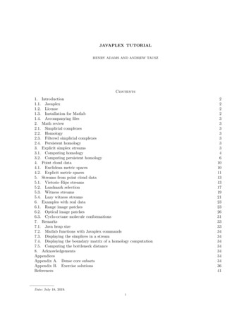
max dimension 3; max filtration value 4; num divisions 1000; point cloud examples.PointCloudExamples.getHouseExample(); stream api.Plex4.createVietorisRipsStream(point cloud, max dimension, .max filtration value, num divisions);The ellipses in the command above should be omitted; they are included only to indicate that this commandcontinues onto the next line.The order of the inputs is createVietorisRipsStream(Z, dmax , tmax , N ). For a Vietoris–Rips stream, the parameter tmax is the maximum possible edge length. Since tmax 4 is greater than the diameter ( 10)of our point cloud, all edges will eventually form.Since dmax 3 we can compute up to second dimensional persistent homology. persistence api.Plex4.getModularSimplicialAlgorithm(max dimension, 2); intervals persistence.computeIntervals(stream);We display the Betti intervals. Parameter options.max filtration value is the largest filtration valueto be displayed; typically options.max filtration value is chosen to be max filtration value. Parameter options.max dimension is the largest persistent homology dimension to be displayed; typicallyoptions.max dimension is chosen to be max dimension - 1 because in a stream with simplices computedup to dimension dmax we can only compute persistent homology up to dimension dmax 1. options.filename ’ripsHouse’;options.max filtration value max filtration value;options.max dimension max dimension - 1;plot barcodes(intervals, options);The file ripsHouse.png is saved to your current directory.14

Check that these plots are consistent with the Vietoris–Rips definition: edges [3

Javaplex is a Java software package for computing the persistent homology of ltered sim- plicial complexes (or more generally, ltered chain complexes), with special emphasis on applications