WIXLIB

2.1.1.2 Hiding Attribute HierarchiesFor many dimensions, you will want the user to navigate hierarchies created for ease of access. Forexample, a customer dimension could be navigated by drilling into country and city before reaching thecustomer name, or by drilling through age groups or income levels. Such hierarchies, covered in moredetail later, make navigation of the cube easier – and make queries more efficient.In addition to user hierarchies, Analysis Services by default creates a flat hierarchy for every attribute ina dimension – these are attribute hierarchies. Hiding attribute hierarchies is often a good idea, becausea lot of hierarchies in a single dimension will typically confuse users and make client queries lessefficient. Consider setting AttributeHierarchyVisible false for most attribute hierarchies and use userhierarchies instead.2.1.1.2.1 Hiding the Surrogate KeyIt is often a good idea to hide the surrogate key attribute in the dimension. If you expose the surrogatekey to the client tools as a ValueColumn, those tools may refer to the key values in reports. Thesurrogate key in a Kimball star schema design holds no business information, and may even change ifyou remodel type2 history. After you create a dependency to the key in the client tools, you cannotchange the key without breaking reports. Because of this, you don’t want end‐user reports referring tothe surrogate key directly – and this is why we recommend hiding it.The best design for a surrogate key is to hide it from users in the dimension design by setting theAttributeHierarchyVisible false and by not including the attribute in any user hierarchies. Thisprevents end‐user tools from referencing the surrogate key, leaving you free to change the key value ifrequirements change.2.1.1.3 Setting or Disabling Ordering of AttributesIn most cases, you want an attribute to have an explicit ordering. For example, you will want a Cityattribute to be sorted alphabetically. You should explicitly set the OrderBy or OrderByAttributeproperty of the attribute to explicitly control this ordering. Typically, this ordering is by attribute nameor key, but it may also be another attribute. If you include an attribute only for the purpose of orderinganother attribute, make sure you set AttributeHierarchyEnabled false andAttributeHierarchyOptimizedState NotOptimized to save on processing operations.There are few cases where you don’t care about the ordering of an attribute, yet the surrogate key isone such case. For such hidden attribute that you used only for implementation purposes, you can setAttributeHierarchyOrdered false to save time during processing of the dimension.2.1.1.4 Setting Default Attribute MembersAny query that does not explicitly reference a hierarchy will use the current member of thathierarchy.The default behavior of Analysis Services is to assign the All member of a dimension as thedefault member, which is normally the desired behavior. But for some attributes, such as the current8

day in a date dimension, it sometimes makes sense to explicitly assign a default member. For example,you may set a default date in the Adventure Works cube like this.ALTERCUBE [Adventure Works]UPDATEDIMENSION [Date], DEFAULT MEMBER '[Date].[Date].&[2000]'However, default members may cause issues in the client tool. For example, Microsoft Excel 2010 willnot provide a visual indication that a default member is currently selected and hence implicitly influencethe query result. This may confuse users who expect the All level to be the current member when noother members are implied by the query. Also, if you set a default member in a dimension with multiplehierarchies, you will typically get results that are hard for users to interpret.In general, prefer explicitly default members only on dimensions with single hierarchies or in hierarchiesthat do not have an All level.2.1.1.5 Removing the All LevelMost dimensions roll up to a common All level, which is the aggregation of all descendants. But thereare some exceptions where is does not make sense to query at the All level. For example, you may havea currency dimension in the cube – and asking for “the sum of all currencies” is a meaningless question.It can even be expensive to ask for the All level of dimension if there is not good aggregate to respond tothe query. For example, if you have a cube partitioned by currency, asking for the All level of currencywill cause a scan of all partitions, which could be expensive and lead to a useless result.In order to prevent users from querying meaningless All levels, you can disable the All member in ahierarchy. You do this by setting the IsAggregateable false on the attribute at the top of the hierarchy.Note that if you disable the All level, you should also set a default member as described in the previoussection– if you don’t, Analysis Services will choose one for you.2.1.1.6 Identifying Attribute RelationshipsAttribute relationships define hierarchical dependencies between attributes. In other words, if A has arelated attribute B, written A B, there is one member in B for every member in A, and many membersin A for a given member in B. For example, given an attribute relationship City State, if the currentcity is Seattle, we know the State must be Washington.Often, there are relationships between attributes that might or might not be manifested in the originaldimension table that can be used by the Analysis Services engine to optimize performance. By default,all attributes are related to the key, and the attribute relationship diagram represents a “bush” whererelationships all stem from the key attribute and end at each other’s attribute.9

Figure 11:1 Bushy attributearelationshippsYou can optimizeoperfoormance by definingdhierarchical relatioonships supported by the data. In this case,ca model namenidentifiees the producct line and subcategory, annd the subcattegory identiffies a categorry. Inother worrds, a single subcategorysiss not found inn more than oneo category. If you redefiine therelationshhips in the atttribute relatioonship editor,, the relationships are cleaarer.Figure 22:2 Redefinned attribuute relationnshipsAttribute relationshipss help performmance in threee significant ways: ot need to go through the key attribute. ThisCross productss between levvels in the hieerarchy do noe during querries.saaves CPU time Aggregations builtbon attribbutes can be reusedrfor quueries on relatted attributess. This savesreesources during processingg and for queeries. Auto‐Exist can more efficiently eliminatee attribute coombinations thattdo not exxist in the datta.Consider thet cross‐prooduct between Subcategorry and Categoory in the twoo figures. In the first, wherre noattribute relationships have been explicitly definned, the enginne must first findfwhich prroducts are inn10

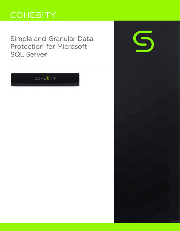
each subcategory and then determine which categories each of these products belongs to. For largedimensions, this can take a long time. If the attribute relationship is defined, the Analysis Servicesengine knows beforehand which category each subcategory belongs to via indexes built at process time.2.1.1.6.1 Flexible vs. Rigid RelationshipsWhen an attribute relationship is defined, the relation can either be flexible or rigid. A flexible attributerelationship is one where members can move around during dimension updates, and a rigid attributerelationship is one where the member relationships are guaranteed to be fixed. For example, therelationship between month and year is fixed because a particular month isn’t going to change its yearwhen the dimension is reprocessed. However, the relationship between customer and city may beflexible as customers move.When a change is detected during process in a flexible relationship, all indexes for partitions referencingthe affected dimension (including the indexes for attribute that are not affected) must be invalidated.This is an expensive operation and may cause Process Update operations to take a very long time.Indexes invalidated by changes in flexible relationships must be rebuilt after a Process Update operationwith a Process Index on the affected partitions; this adds even more time to cube processing.Flexible relationships are the default setting. Carefully consider the advantages of rigid relationships andchange the default where the design allows it.2.1.1.7 Using Hierarchies EffectivelyAnalysis Services enables you to build two types of user hierarchies: natural and unnatural hierarchies.Each type has different design and performance characteristics.In a natural hierarchy, all attributes participating as levels in the hierarchy have direct or indirectattribute relationships from the bottom of the hierarchy to the top of the hierarchy.In an unnaturalhierarchy, the hierarchy consists of at least two consecutive levels that have no attributerelationships. Typically these hierarchies are used to create drill‐down paths of commonly viewedattributes that do not follow any natural hierarchy. For example, users may want to view a hierarchy ofGender and Education.Figure 33: Natural and unnatural hierarchies11

From a performance perspective, natural hierarchies behave very differently than unnatural hierarchiesdo. In natural hierarchies, the hierarchy tree is materialized on disk in hierarchy stores. In addition, allattributes participating in natural hierarchies are automatically considered to be aggregation candidates.Unnatural hierarchies are not materialized on disk, and the attributes participating in unnaturalhierarchies are not automatically considered as aggregation candidates. Rather, they simply provideusers with easy‐to‐use drill‐down paths for commonly viewed attributes that do not have naturalrelationships. By assembling these attributes into hierarchies, you can also use a variety of MDXnavigation functions to easily perform calculations like percent of parent.To take advantage of natural hierarchies, define cascading attribute relationships for all attributes thatparticipate in the hierarchy.2.1.1.8 Turning Off the Attribute HierarchyMember properties provide a different mechanism to expose dimension information. For a givenattribute, member properties are automatically created for every direct attribute relationship. For theprimary key attribute, this means that every attribute that is directly related to the primary key isavailable as a member property of the primary key attribute.If you only want to access an attribute as member property, after you verify that the correct relationshipis in place, you can disable the attribute’s hierarchy by setting the AttributeHierarchyEnabled propertyto False. From a processing perspective, disabling the attribute hierarchy can improve performance anddecrease cube size because the attribute will no longer be indexed or aggregated. This can be especiallyuseful for high‐cardinality attributes that have a one‐to‐one relationship with the primary key. High‐cardinality attributes such as phone numbers and addresses typically do not require slice‐and‐diceanalysis. By disabling the hierarchies for these attributes and accessing them via member properties,you can save processing time and reduce cube size.Deciding whether to disable the attribute’s hierarchy requires that you consider both the querying andprocessing impacts of using member properties. Member properties cannot be placed on a query axis inan MDX query in the same manner as attribute hierarchies and user hierarchies. To query a memberproperty, you must query the attribute that contains that member property.For example, if you require the work phone number for a customer, you must query the properties ofcustomer and then request the phone number property. As a convenience, most front‐end tools easilydisplay member properties in their user interfaces.In general, filtering measures using member properties is slower than filtering using attributehierarchies, because member properties are not indexed and do not participate in aggregations. Theactual impact to query performance depends on how you use the attribute.For example, if your users want to slice and dice data by both account number and account description,from a querying perspective you may be better off having the attribute hierarchies in place andremoving the bitmap indexes if processing performance is an issue.12

2.1.1.9 Reference DimensionsReference dimensions allow you to build a dimensional model on top of a snow flake relational design.While this is a powerful feature, you should understand the implications of using it.By default, a reference dimension is non‐materialized. This means that queries have to perform the joinbetween the reference and the outer dimension table at query time. Also, filters defined on attributes inthe outer dimension table are not driven into the measure group when the bitmaps there are scanned.This may result in reading too much data from disk to answer user queries. Leaving a dimension as non‐materialized prioritizes modeling flexibility over query performance. Consider carefully whether you canafford this tradeoff: cubes are typically intended to be fast ad‐hoc structures, and putting theperformance burden on the end user is rarely a good idea.Analysis Services has the ability to materialize the references dimension. When you enable this option,memory and disk structures are created that make the dimension behave just like a denormalized starschema. This means that you will retain all the performance benefits of a regular, non‐referencedimension. However, be careful with materialized reference dimension – if you run a process update onthe intermediate dimension, any changes in the relationships between the outer dimension and thereference will not be reflected in the cube. Instead, the original relationship between the outerdimension and the measure group is retained – which is most likely not the desired result. In a way, youcan consider the reference table to be a rigid relationship to attributes in the outer attributes. The onlyway to reflect changes in the reference table is to fully process the dimension.2.1.1.10Fast-Changing AttributesSome data models contain attributes that change very fast. Depending on which type of history trackingyou need, you may face different challenges.Type2 Fast‐Changing Attributes ‐ If you track every change to a fast‐changing attribute, this may causethe dimension containing the attribute to grow very large. Type 2 attributes are typically added to adimension with a ProcessAdd command. At some point, running ProcessAdd on a large dimension andrunning all the consistency checks will take a long time. Also, having a huge dimension is unwieldybecause users will have trouble querying it and the server will have trouble keeping it in memory. Agood example of such a modeling challenge is the age of a customer – this will change every year andcause the customer dimension to grow dramatically.Type 1 Fast‐Changing Attributes – Even if you do not track every change to the attribute, you may stillrun into issues with fast‐changing attributes. To reflect a change in the data source to the cube, youhave to run Process Update on the changed dimension. As the cube and dimension grows larger,running Process Update becomes expensive. An example of such a modeling challenge is to track thestatus attribute of a server in a hosting environment (“Running”, “Shut down”, “Overloaded” and so on).A status attribute like this may change several times per day or even per hour. Running frequentProcessUpdates on such a dimension to reflect changes can be an expensive operation, and it may notbe feasible with the locking implementation of Analysis Servicesin a production environment.13

In the following sections, we will look at some modeling options you can use to address these problems.2.1.1.10.1 Type 2 Fast-Changing AttributesIf history tracking is a requirement of a fast‐changing attribute, the best option is often to use the facttable to track history. This is best illustrated with an example. Consider again the customer dimensionwith the age attribute. Modeling the Age attribute directly in the customer dimension produces a designlike this.Figure 44: Age in customer dimensionNotice that every time Thomas has a birthday, a new row is added in the dimension table. Thealternative design approach splits the customer dimension into two dimensions like this.14

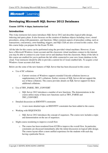
Figure 55: Age in its own dimensionNote that there are some restrictions on the situation where this design can be applied. It works bestwhen the changing attribute takes on a small, distinct set of values. It also adds complexity to thedesign; by adding more dimensions to the model, it creates more work for the ETL developers when thefact table is loaded. Also, consider the storage impact on the fact table: With the alternative design, thefact table becomes wider, and more bytes have to be stored per row.2.1.1.10.2 Type 1 Fast-Changing AttributesYour business requirement may be updating an attribute of a dimension at high frequency, daily, oreven hourly. For a small cube, running Process Update will help you address this issue. But as the cubegrows larger, the run time of Process Update can become too long for the batch window or the real‐time requirements of the cube (you can read more about tuning process update in the processingsection).Consider again the server hosting example: You may want to track the status, which changes frequently,of all servers. For the example, let us say that the server dimension is used by a fact table trackingperformance counters. Assume you have modeled like this.15

Figure 66: Status column in server dimensionThe problem with this model is the Status column. If

Tuning Processing Performance ‐ Processing is the operation that refreshes data in an Analysis Services database. The faster the processing performance, the sooner users can access refreshed data. Analysis Services provides a variety of mechanisms that you can use to influence processing performance,