Transcription
Zhang He (Orcid ID: 0000-0001-7222-9072)Zhang Minghua (Orcid ID: 0000-0002-1927-5405)Fei Kece (Orcid ID: 0000-0001-8520-7278)Ji Duoying (Orcid ID: 0000-0002-1887-887X)Wu Chenglai (Orcid ID: 0000-0002-8397-2424)Zhu Jiawen (Orcid ID: 0000-0002-6174-7234)He Juanxiong (Orcid ID: 0000-0003-3816-9656)Chai Zhaoyang (Orcid ID: 0000-0002-8064-9066)Xie Jinbo (Orcid ID: 0000-0002-3003-9155)Dong Xiao (Orcid ID: 0000-0003-2634-2132)Chen Xueshun (Orcid ID: 0000-0002-4708-1149)Lin Pengfei (Orcid ID: 0000-0003-2361-0066)Lin Zhaohui (Orcid ID: 0000-0003-1376-3106)Liu Hailong (Orcid ID: 0000-0002-8780-0398)Liu Xiaohong (Orcid ID: 0000-0002-3994-5955)Wang Tianyi (Orcid ID: 0000-0002-8726-9197)Wang Zifa (Orcid ID: 0000-0002-7062-6012)Xie Zhenghui (Orcid ID: 0000-0002-3137-561X)Xu Yongfu (Orcid ID: 0000-0002-9925-6756)Yu Yongqiang, yong (Orcid ID: 0000-0001-8596-3583)Zeng Qingcun (Orcid ID: 0000-0002-8237-8802)Zhu Jiang (Orcid ID: 0000-0001-9846-8944)CAS-ESM2: Description and Climate Simulation Performance ofthe Chinese Academy of Sciences (CAS) Earth System Model(ESM) Version 2He Zhang1, Minghua Zhang2 , Jiangbo Jin1, Kece Fei1, Duoying Ji4, Chenglai Wu1, JiawenZhu1, Juanxiong He1, Zhaoyang Chai1, Jinbo Xie3, Xiao Dong1, Dongling Zhang1,Xunqiang Bi6, Hang Cao7, Huansheng Chen8, Kangjun Chen3, Xueshun Chen8, Xin Gao1,Huiqun Hao5, Jinrong Jiang5, Xianghui Kong9, Shigang Li7,10, Yangchun Li8, Pengfei Lin3,Zhaohui Lin1, Hailong Liu3,11, Xiaohong Liu1,12, Ying Shi1,11, Mirong Song3, HuijunWang9,13, Tianyi Wang5, Xiaocong Wang3, Zifa Wang8, Ying Wei14, Baodong Wu15,Zhenghui Xie3,11, Yongfu Xu8, Yongqiang Yu3,11, Liang Yuan7, Qingcun Zeng1, XiaodongZeng1, Shuwen Zhao3, Guangqing Zhou1, Jiang Zhu1 Correspondence to:Minghua Zhang, minghua.zhang@stonybrook.eduThis article has been accepted for publication and undergone full peer review but has not beenthrough the copyediting, typesetting, pagination and proofreading process which may lead todifferences between this version and the Version of Record. Please cite this article as doi:10.1029/2020MS002210 2020 American Geophysical Union. All rights reserved.
1International Center for Climate and Environment Sciences, Institute of Atmospheric Physics,Chinese Academy of Sciences, Beijing, China2School of Marine and Atmospheric Sciences, State University of New York at Stony Brook,Stony Brook, NY, USA3State Key Laboratory of Numerical Modeling for Atmospheric Sciences and GeophysicalFluid Dynamics, Institute of Atmospheric Physics, Chinese Academy of Sciences, Beijing,China4College of Global Change and Earth System Science, Beijing Normal University, Beijing,China5Computer Network Information Center, Chinese Academy of Sciences, Beijing, China6Climate Change Research Center, Chinese Academy of Sciences, Beijing, China7State Key Laboratory of Computer Architecture, Institute of Computing Technology,Chinese Academy of Sciences, Beijing, China8State Key Laboratory of Atmospheric Boundary Layer Physics and Atmospheric Chemistry,Institute of Atmospheric Physics, Chinese Academy of Sciences, Beijing, China.9Nansen‐Zhu International Research Centre, Institute of Atmospheric Physics, ChineseAcademy of Sciences, Beijing, China10Department of Computer Science, ETH Zurich, Switzerland11College of Earth and Planetary Sciences, University of Chinese Academy of Sciences,Beijing, China12Department of Atmospheric Science, Texas A&M University, College Station, USA13Collaborative Innovation Center on Forecast and Evaluation of Meteorological Disasters,Nanjing University for Information Science and Technology, Nanjing, China14Institute of Urban Meteorology, Chinese Meteorological Administration, Beijing, China15Sensetime Beijing, Beijing, ChinaKey Points: The second version of Chinese Academy of Sciences Earth System Model (CAS-ESM2)is described.Strength and weakness of the model simulations from the CMIP6 DECK experiments aredescribed along possible causes.The model has an equilibrium climate sensitivity of 3.4 K with a positive cloud feedbackfrom the shortwave radiation. 2020 American Geophysical Union. All rights reserved.
AbstractThe second version of Chinese Academy of Sciences Earth System Model (CAS-ESM2) isdescribed with emphasis on the development process, strength and weakness, and climatesensitivities in simulations of the Coupled Model Intercomparison Project (CMIP6) DECKexperiments. CAS-ESM2 was built as a numerical model to simulate both the physical climatesystem as well as atmospheric chemistry and carbon cycle. It is a newcomer in the internationalmodeling community to provide sufficiently independent solutions of climate simulations fromthose of other models. Performances of the model in simulating the basic states of the radiationbudget of the atmosphere and ocean, precipitation, circulations, variabilities, and the 20thCentury warming are presented. Model biases and their possible causes are discussed. Strengthincludes horizontal heat transport in the atmosphere and oceans, vertical profile of the AtlanticMeridional Overturning Circulation; weakness includes the double Inter-Tropical ConvergenceZone (ITCZ) and stronger amplitude of the El Niño-Southern Oscillation (ENSO) that are alsocommon in many other models. The simulated the 20th Century warming shares a similardiscrepancy with observations as in several other models—less warming in the 1920s andstronger cooling in the 1960s than in observation—at the time when there was a steep increaseof anthropogenic aerosols. As a result, the 20th Century warming is about 60% of the observedwarming despite that the model simulated a similar slope of warming trend after 1980 toobservation. The model has an equilibrium climate sensitivity of 3.4 K with a positive cloudfeedback from the shortwave radiation.Plain Language SummaryThis paper describes the second version of Chinese Academy of Sciences Earth System Model(CAS-ESM2) along with simulation results from the Coupled Model Intercomparison Project(CMIP6) DECK experiments. Performances of the model in simulating the radiation budget ofthe atmosphere and ocean, precipitation, circulations, variabilities, and the 20th Centurywarming are presented. The simulated the 20th Century warming shares a similar discrepancywith observations as in several other models—less warming in the 1920s and stronger coolingin the 1960s than in observation—at the time when there was a steep increase of anthropogenicaerosols. As a result, the 20th Century warming is about 60% of the observed warming despitethat the model simulated a similar slope of warming trend after 1980 to observation. 2020 American Geophysical Union. All rights reserved.
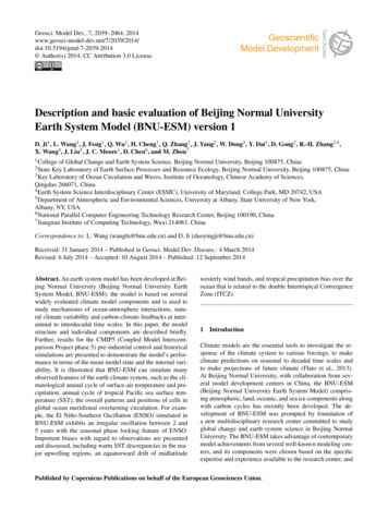
1. IntroductionThe Chinese Academy of Sciences (CAS) Earth System Model version 2 (CAS-ESM2) hasbeen developed to simulate both the physical climate system and the global environmentalprocesses of air pollution and carbon cycle. In developing CAS-ESM, we have set thefollowing priorities. First, we introduce new model parameterizations to provide numericalsimulations that are sufficiently independent from those of other models. Second, the model isbuilt with capability to simulate environmental and ecological systems. The former includesair pollution while the latter vegetation dynamics. Third, wherever possible, physicalparameterizations are designed with placeholders for additional improvements pending onfollow-up diagnostics and evaluations. Additionally, the model is built with a two-way nestingof a regional high-resolution atmospheric model to facilitate the application for simulation andforecasting of regional climate and environmental extreme events.CAS-ESM2 was based on the Institute of Atmospheric Physics (IAP) Atmospheric GeneralCirculation Model (IAP AGCM version 5), the LASG/IAP Climate system Ocean Model(LICOM version 2), the Beijing Normal University/IAP Common Land Model (CoLM), theLos Alamos Sea-Ice Model (CICE version 4), and the Weather Research and Forecast Model(WRF). The model used the Community Earth System Model (CESM) Coupler 7 infrastructure.Additional components are the IAP Vegetation Dynamics Model and the IAP fire modelembedded within the land model; IAP ocean biogeochemistry model embedded within theLICOM ocean model; interactive components through the coupler to CAS-ESM2 of anatmospheric aerosol and chemistry model and various emission models. The model is anewcomer in the community since this is the first time that it is contributing to CMIPsimulations. An earlier version CAS-ESM1 had used IAP GCM4 as the atmospheric model(Zhang et al. 2013) that contained the IAP dynamics but largely the same physicalparameterizations of the Community Atmospheric Model (CAM5). CAS-ESM2 containssignificantly changed physical parameterizations in addition to the IAP dynamical core in theatmospheric model.CAS-ESM has several sister versions of a climate model, the CAS-Flexible Global OceanAtmosphere-Land System model (FGOALS; Li et al. 2020; Guo et al., 2020). FGOALS hascontributed to each phase of the past Coupled Model Intercomparison Project (CMIP). CASESM2 shares the same ocean model as CAS-FGOALS and some features of the dynamicalcore of the atmospheric model in FGOALS-g. It also shares the coupling softwareinfrastructure Coupler 7 of CESM.The purpose of this paper is twofold. One is to describe CAS-ESM2 and its simulation featuresas a reference to a CMIP6 model. Emphasis will be given to remaining biases and possiblecauses. The other is to share our experience in the development of model. The paper isorganized as follows. Section 2 gives a synopsis of the model components. Section 3 describesthe calibration process of the pre-industrial control simulations. Section 4 presents simulationresults of the present-day climate. Section 5 discusses results of climate sensitivity experiments. 2020 American Geophysical Union. All rights reserved.
The last section is a summary. CMIP6 simulation data have been submitted to the ESG grid foranalysis by the community.2. Model Description2.1 Atmospheric modelThe atmospheric component of CAS-ESM2 is IAP AGCM5.0, the fifth generation AGCMdeveloped by IAP. The development of the IAP AGCM started in the early 1980s. It is a globalgrid-point model using finite-difference scheme with a terrain-following σ coordinate. Itspredecessor version IAP AGCM4.1 (Zhang et al., 2013) was released in September 2015 aspart of the CAS-ESM1. Earlier versions of the model used physical parameterizations of theCommunity Atmospheric Model (CAM, e.g., Neale et al., 2010) with some modifications fortunable parameters. The current version is described in the following.a. Dynamical coreThe dynamical core of the atmospheric model IAP AGCM5.0 uses the finite difference methodof Zeng (1983) with two horizontal resolutions, 0.5 degree and 1.4 degree respectively onuniform latitude-longitude grids. The model has three configurations of vertical resolution with35 levels (model top at 2.2 hPa), 60 levels (model top at 2.2 hPa), and 91 levels (model top at0.01 hPa) respectively. For results presented in this paper, the 1.4-degrees and 35-levelresolution configuration is used. Compared to its predecessor IAP AGCM4.1 with 30 levels,the increased vertical layers in IAP AGCM5.0 are mostly located in the lower tropospherebelow 700 hPa (Figure 1), which was designed to improve model performance related toboundary-layer processes.Several novel features of the dynamical core in the IAP AGCM5.0 are inherited from theprevious version 4.0. These include subtraction of the standard atmospheric stratification, inwhich the state variable of temperature is the departure from a prescribed vertical profile ofclimatology; the IAP transform, in which the prognostic variables are atmospheric statevariables weighted by the square root of the surface pressure so that the numerical schemeconserves total available energy instead of total energy; a nonlinear iterative time integrationmethod, and time splitting method. More specific formulations can be found in Zhang et al.(2013). In the IAP AGCM4.1, Fourier filtering is applied to damp the high frequency waves inhigh latitudes. However, the global data communication in the FFT algorithm posed seriouslimitation to the model parallel scalability. Thus, an adaptive leap-format difference isimplemented in the IAP AGCM5.0 instead of FFT filter to achieve high parallel efficiencybased on 3D decomposition (Cao et al., 2020).b. Physical parameterizationsIAP AGCM5.0 uses a two-plume atmospheric convection scheme. The mean vertical velocityin both plumes is calculated by using buoyancy and entrainment as described by the Simpson 2020 American Geophysical Union. All rights reserved.
and Wiggert (1969) equation. The two plumes differ in the parameterizations of theirentrainment/detrainment rates, mass flux closure, and trigger. The deep plume has both anorganized entrainment/detainment and turbulent entrainment/detrainment, conceptually similarto the Tiedtke (1989) scheme, but different in physical assumptions and implementations. Theorganized component in the deep plume is intended to capture buoyance-forced cloud-scalecirculations, while the turbulent component is intended to capture mixing at the lateral surfaceof the plume. The deep plume uses a prognostic closure with the Convective Available PotentialEnergy (CAPE) relaxed toward a quasi-equilibrium condition. It is triggered jointly by CAPE,dCAPE (Xie and Zhang, 2000), and column-integrated precipitable water at a thresholdsaturated value below the level of 750 hPa. The shallow plume uses buoyancy sorting tocalculate entrainment and detainment with Convection Inhibition (CIN) as closure followingPark and Bretherton (2009). It is triggered when the kinetic energy of rising air parcel in theboundary layer is larger to overcome the CIN. The implementation differs from Park andBretherton (2009) in that the lifting forced by large-scale flow and surface heterogneity areadded to the kinetic energy of the parcel. In Park and Bretherton (2009), shallow convection istriggered when the kinetic energy of air parcels at the tail of the subgrid scale distribution ofvertical velocity is larger than the convective inhibition (CIN). We included the large-scalevertical velocity to the subgrid scale vertical velocity. We additionally used the subgriddistribution of terrain and the magnitude of spatial gradients of temperature and humidity atthe resolved scale to form an empirical heterogeneity metric to add to the eddy kinetic energy.Description of the convection scheme and its performance will be presented in a separate paperin this special collection.The turbulence scheme uses the 1st order closure with diagnostic turbulent kinetic energymodified from Bretherton and Park (2009). The two notable changes include the following: (1)Entrainment of cloud-top radiative cooling is calculated by using radiative cooling rate at thetop of the fractional clouds instead of at the whole grid; (2) the impact of mesoscale surfaceinhomogeneity is included in the calculation of the turbulent kinetic energy. Surface mesoscaleinhomogeneity is introduced as a perturbation to the thermodynamic fields by using subgriddistribution of terrain and spatial gradients at the resolved scale.The atmospheric cloud macrophysical scheme uses separate calculations of boundary layerclouds, convective and stratiform clouds above the boundary layer. Within the boundary layer,cloud amount is calculated based on the variances of subgrid variation of liquid water potentialtemperature and total water that are diagnosed from the subgrid scale vertical transportcalculated from the convection and boundary layer scheme. An implicit probability distributionfunction of the subgrid scale variability is used to derive boundary cloud amount and cloudwater, which were based on LES simulations over several climate regimes. Convective cloudamount is parameterized based on convective mass flux and convective vertical velocity aswell as detrained amount of air mass in both the deep and shallow plumes. Stratiform cloudabove the boundary layer uses implicit function of the subgrid scale distribution of temperatureand water vapor that collapses to grid-scale relative humidity, for both water and ice saturationdepending on temperature. Detailed description of the cloud scheme will be submitted in aseparate paper. 2020 American Geophysical Union. All rights reserved.
The cloud microphysical scheme is a modification of the two-moment Morrison and Gettlemen(2008) scheme with several changes: (1) consideration of subgrid scale variability of cloudwater that is dependent on atmospheric stability and model resolution based on measurementsfrom the Atmospheric Radiation Measurement program (ARM) of the U.S. Department ofEnergy (Xie and Zhang, 2015); (2) a new particle size dispersion parameterization based ondata from Liu et al. (2006); (3) inclusion of the impact of spectral dispersion of particle sizedistribution on the collision kernel and in the radiation calculation; (4) inclusion of water vapordeposition onto ice crystals. The cloud microphysical scheme is coupled with the aerosol modelin the same way as in the CAM microphysics with the Modal Aerosol Model (MAM) (Nealeet al., 2013).The radiation scheme uses the RRTMG (Mlawer et al. 1997). The infrared radiation modelRRTMG-LW uses 16 contiguous spectral bands and 140 g-intervals. The shortwave radiationmodel uses the RRTMG-SW with 14 contiguous spectral bands and 112 g-intervals.The orographic gravity wave parameterization is from Xie et al. (2020). It is based on theorographic anisotropy scheme of Kim and Doyle (2005) and Choi and Hong (2017) by allowingthe winds to blow from all directions relative to the terrain orientations.The IAP AGCM5.0 is therefore sufficiently different from other models because of its uniquedynamical core, the new convection and cloud schemes, and many modifications made to otherparameterization schemes adopted from other models2.2 Ocean and sea ice modelsThe ocean component of CAS-ESM2 uses LICOM2.0 (Liu et al., 2012), with -coordinatesand a free surface. The model is formulated on standard latitude-longitude grids at horizontalresolution of approximately 1 globally, increasing to 0.5 meridionally between 10 S and 10 N.There are 30 levels in the vertical direction with 10 m per layer in the upper 150 m. The verticalturbulent mixing scheme is the second-order turbulent scheme of Canuto et al. (2001, 2002).The mesoscale eddy parameterization uses the Gent and McWilliams (1990) scheme with adiffusion coefficient of 1000 m2/s for both the bolus and Redi parts of the isopycnal mixing.Convection is parameterized by convective adjustment (Pacanowski, 1995). Based on originalversion of LICOM2.0, some key modifications have been made: (1) a new sea surface salinityboundary condition is introduced based on the physical process of air-sea flux exchange at theactual sea-air interface (Jin et al., 2017); (2) a new formulation of turbulent air-sea fluxes isintroduced based on Fairall et al. (2003). An evaluation of the ocean model performance canbe found in Lin et al. (2013) and references therein.The sea ice model is modified from the Los Alamos sea ice model Version 4.0 (Hunke andLipscomb, 2008), using the same grid as the oceanic model. The model solves the dynamic andthermodynamic equations for 5 ice thickness categories, with one snow layer and four ice layers. 2020 American Geophysical Union. All rights reserved.
For the dynamic component, we used the elastic-viscous-plastic rheology (Hunke andDukowicz 1997), the mechanical redistribution scheme (Lipscomb et al., 2007) and theincremental remapping advection scheme (Lipscomb and Hunke, 2004). For thethermodynamic component, we used a parameterization with more realistic sea ice salinitybudget as described in Liu (2010).2.3 Land modelThe land component of CAS-ESM2 is the Common Land Model (CoLM; Dai et al. 2003),which was initially developed by incorporating the best features of three earlier land surfacemodels: the Biosphere-Atmosphere Transfer Scheme (BATS; Dickinson et al., 1993), the 1994version of the CAS IAP Land Surface Model (IAP94; Dai and Zeng, 1997) and the NCAR(National Center for Atmospheric Research) Land Surface Model (LSM; Bonan, 1996, 1998).The initial version of CoLM was adopted as the Community Land Model (CLM) for use withthe Community Climate System Model (CCSM; Collins et al., 2006), and later was adopted asthe land component for Beijing Normal University Earth System Model (BNU-ESM, Ji et al.,2014). Currently, the CoLM is radically different from its initial version.Changes include the followings: (1) The two-stream approximation model of radiation transferof the canopy has been improved, with attention to singularities in its solution and with separateintegrations of radiation absorption by sunlit and shaded fractions of canopy (Dai et al., 2004).(2) A photosynthesis-stomatal conductance model is used for sunlit and shaded leavesseparately, and for the simultaneous transfers of CO2 and water vapor into and out of the leaf(Dai et al., 2004). (3) The vertical resolution is increased to 15 vertical soil layers and up to 5snow layers, with which the soil column resolves downwards to 42.1 meters and has the thermalinsulation effects of soil organic matters. The deep soil column and the insulation effects ofsoil organic matter are important to realistically simulate northern high-latitude permafrostextent and its active layer thickness (Lawrence and Slate, 2008). (4) A new frozen soil schemeis introduced by considering the supercooled soil water (Niu and Yang, 2016), which allowsliquid water to coexist with ice in the soil over a wide range of temperatures below 0 C byusing the freezing-point depression equation. The computation of vertical water fluxesconsiders fractional permeable area within a model layer, with the total soil moisture used tocalculate the soil matric potential and hydraulic conductivity. (5) Multi-layer soil organiccarbon (OC) scheme is introduced to describe the cryoturbation and bioturbation effects onvertical soil carbon mixing, which allows the soil carbon generated near the soil surface tomove downwards into colder regions of the soil (Koven et al., 2009). (6) A carbon-nitrogeninteractions scheme is introduced based on LPJ-DyN (Xu and Prentice, 2008). (7) A new frozensoil parameterization is implemented that includes frost and thaw fronts (Gao et al., 2016, 2019).(8) An anthropogenic water use scheme is introduced (Zou et al., 2014, 2015; Zeng et al., 2016,2017). (9) The model has included anthropogenic nitrogen discharge and transport into rivers(Liu et al., 2019).2.4 Dynamic global vegetation model 2020 American Geophysical Union. All rights reserved.
A new dynamic global vegetation model, IAP-DGVM, is coupled with CoLM in the frameworkof CAS-ESM2 (Zhu et al., 2018). The IAP-DGVM classifies land natural vegetation into 12plant functional types with physical, phylogenetic, phenological parameters and bioclimaticlimitations (Zeng et al., 2014). Significant developments in IAP-DGVM included the following:(1) a shrub sub-model (Zeng et al., 2008; Zeng, 2010); (2) a new establishmentparameterization scheme (Song et al., 2016) that enables the model to correctly reproduce theregimes of major terrestrial ecosystems, the dependence of the vegetation distribution onclimate conditions; (3) a process-based fire parameterization of intermediate complexity (Li etal., 2012) to simulate the global fire burned area, fire seasonality and interannual variability.When coupled with CAS-ESM2, IAP-DGVM showed a good performance in simulating globalvegetation distributions and carbon fluxes (Zhu et al., 2018).2.5 Atmospheric aerosol and chemistry modelCAS-ESM2 uses two atmospheric aerosol and chemistry models. One is the IAP Aerosol andAtmospheric Chemistry Model (IAP-AACM; Chen et al., 2015; Wei et al., 2019) which iscoupled with two-way interaction to the IAP AGCM5.0 through the coupler. The other modeluses the three-mode version of modal aerosol mode (MAM3) described in Liu et al. (2012b)and the Model for Ozone and Related chemical Tracers (MOZART) (Emmons et al., 2010;Tilms et al. 2015). The IAP-AACM includes modules to calculate gaseous chemistry,aqueous chemistry, heterogeneous chemistry, dry and wet deposition. For different researchpurposes, two options can be used for gas phase chemistry: the Carbon Bond Mechanism Z(CBMZ; Zaveri and Peters,1999) and a simplified chemistry using the oxidants from CBMZ(Wei et al., 2019). The CBMZ scheme calculates 133 reactions for 53 species to simulate themajor gas-phase reactions for photolysis, ozone production, oxidation of gas pollutants in theatmosphere. The simplified chemistry option uses the oxidants of CBMZ scheme and onlyconsiders the sulfur chemistry.The IAP-AACM also has two versions of aerosol modules to represent the size distribution ofaerosol particles. One is the two-static mode and the other is the size-bin scheme. The twostatic modes include a fine mode to simulate the primary fine particles and secondary particleswith diameters less than 2.5 μm and a coarse mode to simulate primary coarse particles withdiameters in 2.5-10 μm. In this scheme, only the bulk mass concentration of aerosolcomponents is calculated. The dust and sea salt particles are represented by four size bins andthey are calculated online using the schemes developed by Wang et al. (2000) andAthanasopoulou et al. (2008) respectively. The size-bin scheme uses advanced particlemicrophysics (APM; Yu and Luo, 2009) to simulate size distribution of aerosol particles withdry diameters in 0.0012 μm to 12 μm (Chen et al., 2014). The model coupled with this schemehas been used to simulate the spatial-temporal variation of particle number concentration,calculate the aging black carbon (BC) particles, and explore new particle formation events(Chen et al., 2017, 2018, 2019). The IAP-ACCM with the complex chemistry option has beenused in China for air quality and air pollution studies both as a research tool and as anoperational model. The IAP-AACM is coupled to the cloud microphysics model in the sameway as MAM in CAM (Neale et al., 2013). 2020 American Geophysical Union. All rights reserved.
MAM3 described in Liu et al. (2012b) treats both the internal and external mixings of variousaerosol components including BC, OC, sulfate, ammonium, sea salt and mineral dust (Liu etal., 2012b). While anthropogenic aerosol and precursor gas emissions are prescribed, naturalaerosol (dust and sea salt) emissions are interactively calculated in the model. Dust emissionstrongly depends on the near surface wind speed, soil properties and roughness elements. Thedust emission scheme of Shao (2004) is implemented into CAS-ESM2 and dust emission iscoupled to the land model CoLM. The scheme is developed based on wind-erosion physicsassuming that the main mechanisms for dust emission are saltation bombardment andconsequent aggregate disintegration (Shao, 2004). Dust emission occurs in the bare soil whenthe surface wind (in terms of friction velocity) is strong enough to overcome the resistance ofsurface for wind erosion (in terms of threshold friction velocity). Threshold friction velocity iscalculated by adding correction factors from soil moisture (Fecan et al., 1999) and roughnesselements (Raupach et al., 1993) to the idealized threshold friction velocity for dry soils with novegetation cover surrounding. The idealized threshold friction velocity is calculated followingthe scheme of Shao and Lu (2000). In general, CAS-ESM can reasonably simulate the dustemissions over the deserts on the earth and the estimated global dust emission flux is around2640 Tg for piControl experiment. A detailed evaluation of dust simulation in CAS-ESM willbe given in a separate paper in preparation. For the simulations in this paper, the three-modeversion of aerosol module (MAM3) and the MOZART chemistry model are used.2.6 Coupling and configurationThe software framework of CAS-ESM2 is shown in Figure 2, which is based on NCAR’s CPL7(Craig et al., 2012). As with CESM, CAS-ESM2 provides many different model configurations,including both standalone model and various combinations of the individual model components.Two new features in CAS-ESM2 are noted: (1) The mesoscale Weather Research and Forecasts(WRF) model is coupled to atmospheric model IAP AGCM through CPL7 with two-wayinteractions to enable regionally refined climate simulation or one-way downscaling (He et al.2013). (2) The atmospheric aerosol and chemistry model is coupled to the IAP AGCM throughCPL7 rather than embedded within the atmospheric model to facilitate independentdevelopment and maintenance. These two features both involved extension of CPL7 for 3dimensional data mapping and transfer. For the coupling between WRF and the IAP AGCM,the global model generates the lateral condition for the WRF (version 3.6, at present). WRFfeedbacks to the global model by providing relaxation fields of atmospheric state variables forthe IAP AGCM. The coupling of IAP AGCM and WRF is intended for regional high-resolutionshort-term simulations and operational seasonal prediction.The CAS-ESM2 component models’ versions and resolutions for CMIP6 DECK and historicalsimulations are summarized in Table 1. Table 2 summarizes the CAS-ESM2 simulationcampaign described in this paper for CMIP6. The five simulation types followed the CMIP6DECK specifications (Eyring et al., 2016). In the historical and AMIP experiments, the externalforcings are based on CMIP6 data at https://esgf-node.llnl.gov/search/input4mips/. Theseinclude: GHG concentrations for CO2, CH4, N2O, CFC11, and CFC12 from Meinshausen et al. 2020 American Geophysical Union. All rights reserved.
(2017); emissions of short-lived species from Hoesly et al. (2017, 2018) and van Marle et al.(2017); solar forcing from Matthes et al.
CAS-ESM has several sister versions of a climate model, the CAS-Flexible Global Ocean-Atmosphere-Land System model (FGOALS; Li et al. 2020; Guo et al., 2020). FGOALS has contributed to each phase of the past Coupled Model Intercomparison Project (CMIP). CAS-ESM2 shares the same ocean model as CAS-FGOALS and some features of the dynamical