WIXLIB

D. Ji et al.: Description and basic evaluation of BNU-ESMThis paper provides a general description and basic evaluation of the historical climate simulated by BNU-ESM. Particular focus is put on the model structure, the simulated climatology, internal climate variability and terrestrial carboncycle deduced from the piControl and historical simulationssubmitted for CMIP5. The climate response and scenarioprojections in BNU-ESM will be covered elsewhere. The paper is organized as follows. In Sect. 2, a general overview ofBNU-ESM is provided, elaborating on similarities and differences between the original and revised model componentsin BNU-ESM. In Sect. 3, the design of the piControl and historical model experiments is briefly presented, as well as thespin-up strategy. In Sect. 4, the general model performanceis evaluated by using the Taylor diagram (Taylor, 2001). Thefollowing two sections focus on the model performance onsimulating physical climatology and climate variability. Several key modes of internal variability on different timescalesranging from interseasonal to interdecadal are evaluated. Theterrestrial carbon cycle is evaluated in Sect. 7, and particularfocus is put on terrestrial primary productions and soil organic carbon stocks. Finally, the paper is summarized anddiscussed in Sect. 8.22.1Model descriptionAtmospheric modelThe atmospheric component in BNU-ESM is based on Community Atmospheric Model version 3.5 (CAM3.5), which isan interim version of the Community Atmospheric Modelversion 4 (CAM4) (Neale et al., 2010, 2013). Here, the maindifference of the atmospheric component in BNU-ESM relative to the original CAM3.5 model is the process of deep convection. The BNU-ESM uses a modified Zhang–McFarlanescheme in which a revised closure scheme couples convection to the large-scale forcing in the free troposphere insteadof to the convective available potential energy in the atmosphere (Zhang, 2002; Zhang and Mu, 2005a). On the otherhand CAM3.5 adopts a Zhang–McFarlane scheme (Zhangand McFarlane, 1995) modified with the addition of convective momentum transports (Richter and Rasch, 2008), and amodified dilute plume calculation (Neale et al., 2008) following Raymond and Blyth (1986, 1992). BNU-ESM usesthe Eulerian dynamical core in CAM3.5 for transport calculations with a T42 horizontal spectral resolution (approximately 2.81 2.81 transform grid), with 26 levels in thevertical of a hybrid sigma-pressure coordinates and modeltop at 2.917 hPa. Atmospheric chemical processes utilizethe tropospheric MOZART (TROP-MOZART) frameworkin CAM3.5 (Lamarque et al., 2010), which has prognostic greenhouse gases and prescribed aerosols. Note that theaerosols do not directly interact with the cloud scheme sothat any indirect effects are omitted in CAM3.5, as well as 12.2Ocean modelThe ocean component in BNU-ESM is based on the GFDLModular Ocean Model version 4p1 (MOM4p1) released in2009 (Griffies, 2010). The oceanic physics is unchangedfrom the standard MOM4p1 model, and the main modifications are in the general geometry and geography of the oceancomponent. MOM4p1 uses a tripolar grid to avoid the polar singularity over the Arctic, in which the two northernpoles of the curvilinear grid are shifted to land areas overNorth America and Eurasia (Murray, 1996). In BNU-ESM,MOM4p1 uses a nominal latitude-longitude resolution of 1 (down to 1/3 within 10 of the equatorial tropics) with 360longitudinal grids and 200 latitudinal grids, and there are50 vertical levels with the uppermost 23 layers each being10.143 m thick. The mixed layer is represented by the K profile parameterization (KPP) of vertical mixing (Large et al.,1994). The idealized ocean biogeochemistry (iBGC) module is used in BNU-ESM, which carries a single prognostic macronutrient tracer (phosphate, PO4 ), and simulates twomain representative biogeochemical processes, i.e., the netbiological uptake in the euphotic zone due to phytoplankton activity as a function of temperature, light and phosphateavailability, and regeneration of phosphate as an exponentialfunction below the euphotic zone.2.3Sea ice modelThe BNU-ESM sea ice component is the Los Alamos seaice model (CICE) version 4.1 (Hunke and Lipscomb, 2010).The CICE was originally developed to be compatible withthe Parallel Ocean Program (POP), but has been greatly enhanced in its technical and physical compatibility with different models in recent years. In particular, supporting tripolargrids makes it easier to couple with MOM4p1 code. In BNUESM, CICE uses its default shortwave scheme, in which thepenetrating solar radiation is equal to zero for snow-coveredice, that is, most of the incoming sunlight is absorbed nearthe top surface. The visible and near infrared albedos forthick ice and cold snow are set to 0.77, 0.35, 0.96 and 0.69,respectively, slightly smaller than the standard CICE configuration, as they are used as tuning parameters during modelcontrol integration. The surface temperature of ice or snow iscalculated in CICE without exploiting its “zero-layer” thermodynamic scheme, and the “bubbly brine” model based parameterization of ice thermal conductivity is used.2.4Land modelThe land component in BNU-ESM is the Common LandModel (CoLM), which was initially developed by incorporating the best features of three earlier land models: thebiosphere–atmosphere transfer scheme (BATS) (Dickinsonet al., 1993), the 1994 version of the Chinese Academyof Sciences Institute of Atmospheric Physics LSM (IAP94)Geosci. Model Dev., 7, 2039–2064, 2014

2042D. Ji et al.: Description and basic evaluation of BNU-ESM(Dai and Zeng, 1997) and the NCAR Land Surface Model(LSM) (Bonan, 1996, 1998). The CoLM was documented byDai et al. (2001) and introduced to the modeling community in Dai et al. (2003). The initial version of CoLM wasadopted as the Community Land Model (CLM) for use withthe Community Climate System Model (CCSM). The landmodel was then developed separately at NCAR and BNU.Currently, the CoLM is radically different from its initial version and the CLM (Dai et al., 2004; Bonan et al., 2011);including the following: (i) improved two stream approximation model of radiation transfer of the canopy, with attention to singularities in its solution and with separate integrations of radiation absorption by sunlit and shaded fractions of canopy. (ii) A photosynthesis-stomatal conductancemodel for sunlit and shaded leaves separately, and for the simultaneous transfers of CO2 and water vapor into and outof the leaf. (iii) Lund–Potsdam–Jena (LPJ) model (Sitch etal., 2003) based dynamical global vegetation model and terrestrial carbon cycle, and LPJ-DyN (Xu and Prentice, 2008)based scheme on carbon-nitrogen cycle interactions. Notethat in all BNU-ESM’s CMIP5 and GeoMIP simulations,carbon-nitrogen cycle interactions are turned off as the nitrogen cycle has not yet been fully evaluated.2.5Figure 1. The global mean TOA and surface net radiation flux,global mean SST over the piControl simulation period. The blacklines are linear regressions.Component couplingThe coupling framework of BNU-ESM is largely basedon the coupler in NCAR CCSM3.5 (an interim version ofNCAR CCSM4), with changes on grid mapping interpolation to allow for the identical tripolar grids used in both oceanand sea ice components. The time evolution of the wholemodel and communication between various component models are all synchronized and controlled by the coupler in theBNU-ESM. Since MOM4p1 and CICE4.1 are both ArakawaB-grid models, the coupling between them is efficient, andthe exchanged fields need no transformation or additionaltreatment (e.g., vector rotation, grid remapping, grid-pointshifting, etc.). The different model components are run simultaneously from their initial conditions. The atmosphericcomponent uses a 1 h time step for atmospheric radiation and20 min time step for other atmospheric physics. The ocean,sea ice and land components have a 2 h, 1 h and 30 min timestep, respectively, while direct coupling occurs hourly amongatmospheric, sea ice and land components, and daily with theocean component without any flux adjustment.All biogeochemical components are driven by the physical climate with the biogeochemical feedback loops combined. The terrestrial carbon cycle module determines theexchange of CO2 between the land and the atmosphere. It iscoupled to the physical climate through the vegetation distribution and leaf area index, which affects the surface albedo,the evapotranspiration flux and so on. As with the terrestrialcarbon cycle module, the ocean biogeochemistry module calculates the ocean-atmosphere exchange of CO2 , and both areGeosci. Model Dev., 7, 2039–2064, 2014coupled with the TROP-MOZART framework in the atmospheric component to form a closed carbon cycle.3ExperimentsFollowing CMIP5 specifications (Taylor et al., 2009), BNUESM has performed all CMIP5 long-term core experimentsand part of the tier-1 experiments. The CMIP5 specification requires each model to reach its equilibrium states before kicking off formal simulations, especially for long-termcontrol experiments. BNU-ESM adopted a two-step spin-upstrategy to achieve model equilibrium. Firstly, the land component including vegetation dynamics and terrestrial carboncycle, and the ocean component including biogeochemicalmodule were separately spun-up to yield an initial estimateof equilibrium states. In these off-line integrations of the firststep spin-up, surface physical quantities such as winds, temperature, precipitation, moisture, and radiation flux are takenas the climatology of a pre-industrial run of the fully coupledBNU-ESM with carbon cycles turned off. Then, the resultantequilibrated physical and carbon cycle states were fed intothe coupled model as initial conditions to do on-line spin-upto achieve final equilibrium states. During the second stage,the coupled model was forced with constant external conditions as specified for CMIP5 pre-industrial control simulation as stated below.www.geosci-model-dev.net/7/2039/2014/

D. Ji et al.: Description and basic evaluation of BNU-ESM2043Table 1. Observationally based reference data sets.Variable ture [ C]ERA-Interima /JRA-55bzonal wind [m s 1 ]meridional wind [m s 1 ]geopotential height [m]specific humidity [kg kg 1 ]TOA outgoing long-wave radiation [W m 2 ]TOA net shortwave radiation [W m 2 ]long-wave cloud radiative forcing [W m 2 ]shortwave cloud radiative forcing [W m 2 ]total precipitation [mm day 1 ]total cloud cover [%]precipitable water [g kg 1 ]sea level pressure [Pa]surface (10 m) zonal wind speed [m s 1 ]surface (10 m) meridional wind speed [m s 1 ]sea surface temperature [ C]ocean surface zonal wind stress [Pa]ocean surface meridional wind stress [Pa]ocean surface latent heat flux [W m 2 ]ocean surface sensible heat flux [W m 2 ]land surface latent heat flux [W m 2 ]land surface sensible heat flux [W m 2 ]gross primary productivity [kg m 2 s 1 ]surface CO2 flux [kg m 2 s 1 ]ERA-Interima /JRA-55bERA-Interima /JRA-55bERA-Interima /JRA-55bERA-Interima /MERRAcERBEd /CERES-EBAFeERBEd /CERES-EBAFeERBEd /CERES-EBAFeERBEd /CERES-EBAFeGPCPf /CMAPgISCCP-D2h /CLOUDSATiRSS(v7)j /NVAPkERA-Interima /JRA-55bERA-Interima /JRA-55bERA-Interima /JRA-55bHadISSTl /OISST(v2)mERA-Interima /NOCSnERA-Interima /NOCSnERA-Interima /NOCSnERA-Interima /NOCSnERA-Interima /FLUXNET-MTEoERA-Interima /FLUXNET-MTEoFLUXNET-MTEoLDEOp200, 850 hPa200, 850 hPa200, 850 hPa500 hPa400, 850 hPaequatorward of 60 equatorward of 60 ocean onlyocean onlyocean onlyocean only, equatorward of 50 ocean onlyocean onlyocean onlyocean onlyland onlyland onlyland onlyocean onlya ERA-Interim (Dee et al., 2011); b JRA-55 (Ebita et al., 2011); c MERRA (Rienecker et al., 2011); d ERBE (Barkstrom, 1984); e CERES-EBAF (Loeb et al., 2009); f GPCP(Adler et al., 2003); g CMAP (Xie and Arkin, 1997); h ISCCP-D2 (Rossow and Schiffer, 1999; Rossow and Dueñas, 2004); i CLOUDSAT (L’Ecuyer et al., 2008); j RSS(Wentz, 2000, 2013); k NVAP (Simpson et al., 2001); l HadISST (Rayner et al., 2003); m OISST (Reynolds et al., 2002); n NOCS (Josey et al., 1999); o FLUXNET-MTE(Jung et al., 2011); p LDEO (Takahashi et al., 2009).In this paper, we focus on the 559 year (from model year1450 to 2008) pre-industrial control simulation (piControl)and 156 year historical simulation representing the historical period from year 1850 to 2005. The piControl simulation is integrated with constant external forcing prescribedat 1850 conditions (the solar constant is 1365.885 W m 2 ,the concentrations of CO2 , CH4 , N2 O are 284.725 ppmv,790.979 ppbv, and 275.425 ppbv respectively, CFC-11, CFC12 and volcanic aerosols are assumed to be zero). In termsof energy balance and model stability, the global mean topof-atmosphere (TOA) net radiation flux over piControl period is 0.88 W m 2 , while the global mean surface net radiation flux is 0.86 W m 2 . The global mean sea surface temperature over piControl period is 17.69 C with a warmingdrift of 0.02 C per century (Fig. 1). The historical simulation is initialized with the model states of 1850 year from piControl simulation, and forced with natural variation of solar radiation (Lean et al., 2005; Wang et al., 2005), anthropogenic changes in greenhouse gases concentrations, stratospheric sulphate aerosol concentrations from explosive volcanoes (Ammann et al., 2003), and aerosol concentrations ofsulfate, black and organic carbon, dust and sea salt accordingwww.geosci-model-dev.net/7/2039/2014/to Lamarque et al. (2010). Note that there is no land-coverchange related to (anthropogenic) land use because the vegetation distributions evolve according to the model-simulatedclimate, and the areal fraction of non-vegetated regions (lake,wetland, glacier and urban) are fixed according to the GlobalLand Cover Characterization (GLCC) Database. Therefore,changes in physical and biogeochemical properties of thevegetation due to actual land-cover changes are excluded bydesign.4General model performanceTo systematically evaluate the general performance of BNUESM, we use the Taylor diagram (Taylor, 2001; Gleckler etal., 2008), which relates the “centered” root-mean square(RMS) error, the pattern correlation and the standard deviation of particular climate fields. We selected 24 fields(Table 1) and compared model simulations with two different reference data sets (only one data set was available forgross primary production over land and surface CO2 fluxover ocean). The selection rationale for the fields and reference data sets follows Gleckler et al. (2008), where mostGeosci. Model Dev., 7, 2039–2064, 2014

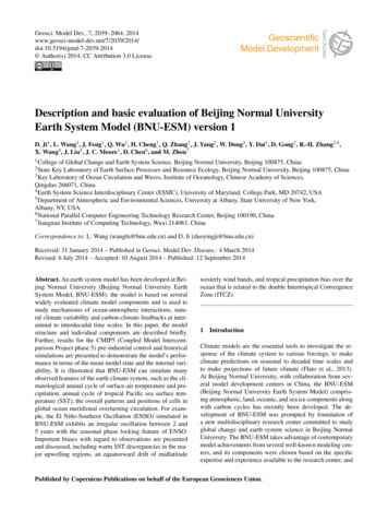
2044of reference data sets are briefly described. One notabledifference is that we use ERA-Interim (Dee et al., 2011)and JRA-55 (Ebita et al., 2011) reanalysis data instead ofERA40 and NCEP to reflect recent advances in reanalysissystems. We use estimates of specific humidity from National Aeronautics and Space Administration (NASA) Modern Era Retrospective analysis for Research and Applications(MERRA, Rienecker et al., 2011) instead of the AtmosphericInfrared Sounder (AIRS) experiment, as Tian et al. (2013)indicated MERRA specific humidity probably has a smalleruncertainty than the AIRS data set. The International Satellite Cloud Climatology Project (ISCCP, Rossow and Schiffer, 1999; Rossow and Dueñas, 2004) D2 and CLOUDSAT(L’Ecuyer et al., 2008) data sets are used to examine the total cloud cover. The Clouds and the Earth’s Radiant EnergySystem – Energy Balanced and Filled (CERES-EBAF) dataset (Loeb et al., 2009) is used instead of the CERES observations, because the energy balanced characteristics of CERESEBAF made it more suitable for the near balanced energeticsof the earth system. Two carbon cycle fields (gpp and fgco2)were added to fill the gap between climate system modeland earth system model. The reference data used to examine gross primary production (gpp) over land is FLUXNETModel Tree Ensembles (FLUXNET-MTE) estimates (Jung etal., 2011), which are restricted to vegetated land surface. Thereference data used to examine surface CO2 flux over ocean(fgco2) is from Lamont–Doherty Earth Observatory (LDEO,Takahashi et al., 2009), this climatology data set was createdfrom about 3 million direct observations of seawater pCO2around the world between 1970 and 2007.Figure 2 shows six climatological annual-cycle space-timeTaylor diagrams for the 24 selected fields in Table 1 for thetropical (20 S–20 N) and the northern extra-tropical (20–90 N) zones. It is clear from Fig. 2 that the accuracy ofthe model varies between fields and domains. Some simulated fields over the northern extra-tropics have correlationswith the reference data of greater than 0.95 (e.g., zg-500hPa,ta-850hPa, rlut, rsnt, tos), and most of fields have correlations with the reference data of greater than 0.8, whereasone field has much lower correlation of 0.38 (fgco2 over thenorthern extra-tropics). The amplitude of spatial and temporal variability simulated by the model is reasonably close tothat of observationally based reference data. The normalizedstandard deviations between the simulation and the referencedata of most fields have a bias of less than 0.25, and several fields have a bias of less than 0.1 (e.g., ta-850hPa, hus850hPa, rlut, rsnt, psl, tos). One outlier in Fig. 2 (NHEX G3and TROP G3) is the sensible heat flux over ocean (hfss) examined with National Oceanography Centre, Southampton(NOCS) reference data (Josey et al., 1999). The model showsbetter skills when compared to ERA-Interim reanalysis, although the pattern correlations against two reference datasets are both of about 0.6. Previous studies suggest that thereare large uncertainties in NOCS data set, and their pattern hasbetter agreement with reanalysis products than the magnitudeGeosci. Model Dev., 7, 2039–2064, 2014D. Ji et al.: Description and basic evaluation of BNU-ESMFigure 2. Multivariate Taylor diagrams of the 20th century annualcycle climatological (1986–2005) for the tropical (20 S–20 N,TROP) and the northern extra-tropical (20–90 N, NHEX) zones.Each field is normalized by the corresponding standard deviation ofthe reference data, which allows multiple fields to be shown in eachsub-figure. Red/Blue markers represent the simulation field evaluated against the Reference1/Reference2 data defined in Table 1.of their fluxes (e.g., Taylor, 2000). In general, most of fieldsover the tropics are closer to reference data than those overthe northern extra-tropics in Taylor diagrams, but some fieldswith relatively high correlations in the northern extra-tropicshave a lower skill in the tropics. These features are consistentwith Gleckler et al. (2008).55.1Climatology in the late 20th centuryAtmospheric mean stateFigure 3 shows the zonally averaged mean atmospheric temperature, zonal wind and specific humidity for the historical simulation of the BNU-ESM and its deviations from theERA-Interim reanalysis (Dee et al., 2011). The air temperature in the troposphere is in general cold for both borealsummer and winter, especially during the boreal summer(Fig. 3a). Near the polar tropopause (about 250 hPa) thereis a relatively large cold bias up to 8 K over the Arctic duringJJA, and up to 10 K over the Antarctica during December–February (DJF). This tropospheric cold bias is one common problem in many CMIP5 models (Charlton-Perez etal., 2013; Tian et al., 2013). In the lower polar tropospherewww.geosci-model-dev.net/7/2039/2014/

D. Ji et al.: Description and basic evaluation of BNU-ESMFigure 3. Zonally averaged air temperature (a), zonal wind (b) andspecific humidity (c) climatology from BNU-ESM historical simulation (black contours) and bias relative to the ERA-Interim climatology (color fi

ESM, and the model has received comprehensive eval-uations. For example, Wu et al. (2013) evaluated the precipitation-surface temperature (P-T) relationship of BNU-ESM among 17 models in CMIP5 and found BNU-ESM has better ability in simulating P-T pattern correla-tion than other models, especially over ocean and tropics.