Transcription
Machine Scheduling Performance withMaintenance and FailureY. Guo4, A. Lim¹, B. Rodrigues², S. Yu³¹Department of IELM, Hong Kong University of Science andTechnology, Clear Water Bay, Kowloon, Hong Kong²School of Business, Singapore Management University,50 Stamford Road, Singapore 178899³School of Computing, National University of Singapore,3 Science Drive 2, Singapore 1175434Department of Computer Science, Cornell University,Ithaca, New York, USA 14853AbstractIn manufacturing control, machine scheduling research has mostly dealt withproblems either without maintenance or with deterministic maintenance when no failurecan occur. This can be unrealistic in practical settings. In this work, an experimentalmodel is developed to evaluate the effect of corrective and preventive maintenanceschemes on scheduling performance in the presence machine failure where thescheduling objective is to minimize schedule duration. We show that neither scheme isclearly superior, but that the applicability of each depends on several system parametersas well as the scheduling environment itself. Further, we show that parameter values canbe chosen for which preventive maintenance does better than corrective maintenance.The results provided in this study can be useful to practitioners and to system or machineadministrators in manufacturing and elsewhere.Key Words: machine scheduling, experiments, manufacturing control, maintenance1
1. IntroductionIn machine scheduling control, good bounds are available for the problem ofminimizing schedule durations, or the makespan. Graham [8] provided a worst-casebound for the approximation algorithm, Longest Processing Time, and Coffman, Gareyand Johnson [6] provided an improved bound using the heuristic, MULTIFIT. Bycombining these, Lee and Massey [13] were able to obtain an even tighter bound. Thesestudies, however, assumed the continuous availability of machines, which may not bejustified in realistic applications where machines can become unavailable due todeterministic or random reasons.It was not until the late 1980’s that research was carried out on machine schedulingwith availability constraints. In a study, Lee [15] considered the problem of parallelmachine scheduling with non-simultaneous available time. In another work, Lee [14]discussed various performance measures and machine environments with singleunavailability. For each variant of the problem, a solution was provided using apolynomial algorithm, or it was shown that the problem is NP-hard. Turkcan [24]analyzed the availability constraints for both the deterministic and stochastic cases. Qi,Chen and Tu [21] conducted a study on scheduling the maintenance on a single-machine.The reader is referred to Turkcan [24] for a detailed literature review of machinescheduling with availability constraints. Other work on scheduling with maintenance isavailable, but with different scheduling environments and/or objectives. Lee and Liman[16] studied single-machine flow-time scheduling with maintenance while Kaspi andMontreuil [12] attempted to minimize the total weighted completion time in two2
machines with maintenance. Schmidt [23] discussed general scheduling problems withavailability constraints, taking into account different release and due dates.These studies addressed the problem of maintenance, but in a limited way. Theyeither considered only one deterministic maintenance (or availability) constraint ormaintenance without machine failures. The results, however, are inadequate for solvingreal problems. In industrial systems, machines can fail due to heating or lack oflubrication, for example; in computer systems, the Internet is a typical example of systeminstability and breakdowns due to both hardware and software problems. In such cases,maintenance needs to be carried out, either periodically or after failure. Yet, even withmaintenance, failures are not completely eliminated. Further, the overall performance,rather than the worst-case performance, is of greater relevance to the users andadministrators of these systems.In this work, we address this need and study the average or expected performance ofmachine scheduling with both maintenance and failures. Since maintenance as well asfailure are everyday occurrences in industry, this study is particularly relevant topractitioners and systems administrators.1.1 Scope and PreliminariesWe first discuss the scheduling environment, and the rules and maintenanceschemes used in this study. For basic notations and definitions, see, for example, Pinedo[20]Scheduling environment: This study focuses on two areas: one, on single-machinescheduling, and the other on multiple (and identical) machine scheduling. All jobs are3
released at zero time. The objective is to minimize the makespan. In short, the schedulingenvironments studied are described as 1 Cmax and Pm Cmax.Scheduling rules: In view of the simple structure in the problem, we use two schedulingrules, namely Longest Processing Time first (LPT) and Service In Random Order(SIRO), both of which are list scheduling rules. LPT sorts all jobs into a list in nonincreasing order; SIRO generates a list of random permutation of all jobs, and if the inputjobs are already in random order, then there is no need to generate another randompermutation. Each time a machine is freed, the job at the beginning of the list is assignedto the machine.Maintenance schemes: We first define an “interruption” to be a stoppage of a machineeither due to machine failure or to maintenance. There are two maintenance schemes ingeneral: corrective maintenance (CM) and preventive maintenance (PM). CM executesmaintenance only after each failure. It is assumed (regardless of the maintenance scheme)that the time spent on maintenance after failure is linearly proportional to the timebetween two failures. PM executes maintenance after a fixed period of time from the lastinterruption, and after failures. It is assumed that in PM the time spent on maintenanceafter a fixed period of time is a constant.The objective of this work is to evaluate the performance of CM and PM with ascheduling rule LPT or SIRO in the environment 1 Cmax and Pm Cmax. In the following,how the problem is modeled is discussed in Section 2, and experiment design isexplained in Section 3. Following this, single-machine experiments are developed insection 4 and multiple-machine experiments in Section 5. Conclusions drawn for theexperiments are provided in Section 6. In Section 7, the work is summarized.4
2. Modeling the Problem2.1 System modeling Most aspects of system modeling are straightforward exceptmachine maintenance and failure. In CM, a Random Number Generator (RNG) is used togenerate the Time Between Failures (TBF). The time between failures follows normaldistribution with a specified Mean Time To Failure (MTTF) and standard deviation std.The philosophy behind this is that most TBF values will be in the neighborhood of amean time, and extremely long or short TBFs are unlikely. The Maintenance Time (MT)is a linear factor of the duration between failures. In PM, the failure time is generated inthe same way (see section 4.3). Each interruption is caused by the smaller of the fixedperiod for maintenance and TBF. The MT after fixed time is a specified constant, and theMT after failure is a linear factor of the Time Between Interruptions (TBI). Figure 1illustrates this:TBF(working)failurefixed timemaintenancestartsMT ing)failuremaintenancedoneFigure 1 (a)TBI(working)MT afterfixed timeTBI(working)MT afterfailureTBI(working)Figure 1 (b)Figure 1 (a) and (b) are sample time lines for corrective maintenance and preventivemaintenance, respectively5
2.2 Job modeling Jobs are described by their processing times. The processing timesfollow an exponential distribution with a specified mean and are generated by a randomnumber generator. All jobs are non-resumable, that is to say, if some job is interruptedbefore completion, whether because of machine failure or maintenance, it must beprocessed again from the very beginning after the machine restarts.3. Experiment DesignHere, we provide the key characteristics of the experiment design. These are theperformance metrics, parameters, factor and levels and lastly, experimental procedures.For related and general descriptions see [1], [2], [3], [4], [9], [10], [11], [17], [18], [19],[22].3.1 Performance Metrics The performance metric used is the scheduling objective itself,the makespan (Cmax), which is the completion time of the job that finishes last. A smallCmax indicates balanced load on multiple-machines and is consequently desirable.Another metric we adopt is the Total Maintenance Time (TMT). In CM, TMT onlyconsists of the maintenance time used after failure, whereas in PM, it consists of themaintenance time used after fixed period as well as after failure. The maintenance time isactually akin to an overhead, so that a smaller TMT is preferable.3.2 Parameters There are roughly three types of parameters that can affect the aboveperformance metrics. The first kind is system and workload parameters: the number ofmachines m, the number of jobs n, and the mean processing time of jobs u. Parameters ofthis kind are usually not in the control of the system or machine administrator, or at least,6
cannot be changed or modified at discretion. The second kind is scheduling parameters:the scheduling rule in this case – whether we choose SIRO or LPT. This parameter is atfull control of the administrator, and can be changed with little effort. The last type ofparameters are maintenance parameters. In CM, we have three maintenance parameters.The first is the mean time to failure (denoted by MTTFc, where the “c” subscriptindicates “corrective”), which is negatively related to failure rate. The second is thestandard deviation, std, of the time to failures (MTTFc and std together determine thenormal curve from which we compute time between failures). The third is the linearfactor k, which specifies how much maintenance time is needed for each period of timebetween failures, i.e. MT k TBF. All three are usually decided by the workingenvironment and cannot be easily changed. In PM, we also have the above-mentionedthree parameters. The Mean Time To Failure in PM (denoted by MTTFp) is assumed tobe larger than MTTFc, because more diligent maintenance is expected to result in asmaller failure rate and thus a larger MTTFp. (MTTFp will be discussed again in this subsection) The standard deviation std and the linear factor k in PM are assumed to be thesame as in CM. Besides the three, we use other parameters for PM. In PM, maintenanceis carried out at fixed intervals, and the time between two maintenance events is calledFixed Maintenance Period (FMP). The parameter, a, is a linear factor between FMP andMTTFc, i.e., FMP a MTTFc. Fixed interval maintenance takes a fixed amount oftime, and this time is called Fixed Maintenance Time (FMT). FMT is expected to besmaller than the mean of MT in CM, because the maintenance is carried out whenmachines are still in working condition and therefore less maintenance needs to be done.However, there is also no reason why this cannot be greater than the mean of MT. The7
parameter, b, is a linear factor between FMT and E(MT), i.e., FMT b E(MT), whereE(.) is the expectation function. We use another parameter c, to describe the linearrelationship between MTTFc and MTTFp, i.e., MTTFp c MTTFc. In summary, wehave five parameters in PM: std, k, a, b and c. The parameters a, b, and c can becontrolled: to vary a, corresponds to vary the FMP, is easily done; to vary b,corresponding to varying FMT, can be done by selecting error-prone parts of the machineto maintain, and ignoring stable parts; to vary c is similar to varying b.Figure 2 is shows parameters and performance metrics involved and Table 1 is asummary of all notation and parameters, their meanings, and values taken or levels(discussed next).CMSystem and workloadparametersMaintenance parametersMTTFc, std, kPMMTTFp (or c), std, kFMP (or a),FMT (or b)m, n, uSchedulingparametersLPT or SIROPerformance metricCmax, TMTFigure 2 The relationship between parameters and performance metricsValue or levels (if any)NameSymbolMeaningtotal epreventivemaintenanceTMTthe sum of all maintenance performance metrictime usedthe completion time of the performance metriclast finished jobmaintaining after failureCmaxCMPMmaintaining after failureand after fixed period8
longest processing LPTtime firstservice in random SIROordermmthe number of machines1 (1 Cmax), 10 (Pm Cmax)nnthe number of jobs10000 (1 Cmax)100000 (Pm Cmax)uumean processing time10mean time tofailure correctivemean time tofailure preventivestandard deviationMTTFc1000time betweenfailuretime betweeninterruptionmaintenance timeTBFmean of the time betweenfailures in CMmean of the time betweenfailures in PMstandard deviation of thetime between failuresthe amount of timebetween two failuresthe amount of timebetween two interruptionsmaintenance time tenancesmaintenance time at a fixedintervallinear factor of MT fromTBI or TBFlinear factor of FMP fromMTTFclinear factor of FMT fromthe mean of MT in CMlinear factor of MTTFcfrom MTTFpMTTFpstdTBIMTfixed maintenance FMPperiodfixed maintenance FMTtimekkaabbccdoing the longestprocessing time job firstdoing the jobs randomlydepending on c200depending on MTTFc orMTTFp, and stddepending on MTTFpand stddepending on kconstant, depending on aconstant, depending on b0.010.2, 0.4, 0.6, , 2.8, 3.00.2, 0.4, 0.6, , 1.8, 2.01.00, 1.25, 1.50, , 2.75,3.00Table 1 Summary of terminology and parameters used3.3 Factors and Levels Factors are selected parameters that are believed to havesignificant impact on the performance, or that are at the control of end users and need tobe optimized. Levels are a set of values taken by each factor. In our case, we will select9
parameters that can somehow be changed or modified by the machine administrators. InCM, all parameters except scheduling rules are inherently determined by the system andworkload, which are not easily changeable. In PM, in addition to scheduling rules, theparameters a, b, and c can be modified by the administrator to different extents.Therefore, a, b, c can be selected and scheduling rules taken to be our factors.The factor a corresponds to FMP. Because of it is easy to change, its level will rangefrom very small, 0.2, to a reasonably large value 3, with a step size of 0.2. We choose a torange from 0.2 to 3 because FMP a MTTF, and we want to make FMP and MTTFapproximately comparable, otherwise either preemptive maintenance or failure wouldalmost never happen in the PM model.The factor b corresponds to FMT, which is expected to be smaller than E(MT),because maintaining the machine at working condition is easier than doing so at machinefailures. But we do not exclude the possibility of FMT E(MT). Meanwhile, we notethat FMT is not as flexible as FMP: it is varied by maintaining different components ofthe machines. Usually error-prone components are maintained periodically and otherstable components are attended only after their failure. By doing so, we can shorten FMT.Based on the above, the level of b will be taken to range from 0.2 to 2.0, with each step of0.2.The factor c corresponds to MTTFp, which is expected to be larger than MTTFc,because after all, this is why we may want to adopt PM. MTTFc is around the same levelof flexibility as FMT for exactly the same reason. Usually error-prone components aremaintained periodically because this will improve c more effectively than othercomponents. Hence, the level of c will range from 1.0 to 3.0, with step-size of 0.25.10
Here, the scheduling rule can be either LPT or SIRO, and our objective is to comparethe performance of CM and PM in machine scheduling with machine failures andobserve how much parameters and factors affect performance.3.4 Experiment Procedure Because of the large number of factors and their levels, it isimpossible and impractical to plan a full experiment. For each environment (single ormultiple-machines), we conducted the experiment in the following way. First, we ran testcases on CM with LPT and SIRO respectively. The rule yielding in better results wasapplied in PM. Then, at each level of a factor, we ran the same test cases on PM,compared the results with that of CM, and observed how performance varied with eachfactor. For each level of each factor, there were 100 test cases.3.5 The necessity of experiments An experimental approach is taken in this study forseveral reasons. First, practitioners are more interested in average-case performance thanthe worst-case performance, whereas traditional analysis focuses on the worst cases andcan provide only limited insights to the average case. Second, taking machine failure intoaccount complicates the problem by introducing random variables with known orunknown distributions. For example, the time between failures is a normal randomvariable, but the failure count (the number of failures) and the wasted time due tointerruption have unknown distributions and are not amenable to the simple worst-caseand statistical analysis. Third, in order to compare the two maintenance schemes, we needto vary some parameters and factor levels, which is almost impossible by analytical11
characterizations alone. Only by running tests and analyzing the collected data is itpossible to observe the performance in various situations.3.6 Reproducibility Since reproducibility is a crucial part of any experimental study, wedescribe the random number generator (RNG) used in the experiments. A Java softwarepackage, COLT, consisting of six libraries for scientific and technical computing, is index.html). Ranecu, which is an advanced multiplicative linearcongruential random number generator with a period of approximately 1018, is used.Using this, we generated all job processing times and the time between failures. Testcases were run on a Pentium III (600MHz) with 128MB memory and programs werewritten in Java, and compiled and run with Java sdk1.4.0 and COLT1.0.3.Theexperiments’ results are obtained in very short run time.4. Single-machine Experiments4.1 Selecting scheduling rule For single-machine scheduling minimizing Cmax with nomaintenance and failure, any non-delay schedule is an optimal solution. Data on Cmax andTMT were collected from 100 test cases using a CM maintenance scheme. A 5%significance hypothesis testing was carried out to confirm or reject the conjecture. Table2 shows the sample means and standard deviations of Cmax and TMT respectively of 100test cases used.12
e 2 Summary of data from 100 test cases in single-machine environmentFrom the test data and the results of hypothesis testing, we conclude with 5% significancelevel that there is a negligible difference between the scheduling rule SIRO and LPT interms of Cmax and TMT. However, in LPT the jobs are first to be sorted in non-decreasingprocessing time, so it takes more time and computational cost; whereas in SIRO, jobs cansimply be processed in input order because they are randomly generated, and thus are inrandom order. Therefore, SIRO is preferable and is used here for the single-machineenvironment.4.2 Effects of the factors a, b and cFactor a: Before experimentation, we first analyzed how performance will be affected bya using PM. Since a is positively proportional to FMP, a small a indicates frequentmaintenance, which can reduce failure rate but also incur more maintenance time. So asmall a is expected to offset the effect of increased MTTFp and even cause performanceto be worse off than that using CM. On the other hand, if a becomes large, theperformance of PM will converge to that of CM, because failure frequently occurs beforefixed-time maintenance is carried out. Based on the preliminary analysis, we inferred thatthere should be an optimal value of a which will maximize the performance difference13
between PM and CM. Experiments with various values of a were performed to collectdata of Cmax and TMT for CM and PM respectively; meanwhile, other parameters wereset as shown in Table 1, and factor b and c fixed at 0.6 and 2 respectively. Two graphswere plotted for the test data.In Figure 3(a), the x-axis corresponds to the a value, and the y-axis, called the ratio ofCmax gain, corresponds to the values (Cmax,CM – Cmax,PM)/Cmax,CM. In Figure 3(b), the xaxis is still the a value, and the y-axis, called the ratio of TMT gain, corresponds to thevalues (TMTCM – TMTPM)/TMTCM. Above the dash-dot line at 0, PM outperforms CM,and vice versa. From the graphs, we see that the two curves have similar shape: when a isless than 1, CM is better; when a is between 1.5 and 2, the ratio reaches maximum,indicating the optimal value of a for PM; when a is greater than 2, the ratio converges to0, indicating the close performance of CM and PM. There are several points worth notinghere. First, the two curves are similar because in single-machine scheduling, Cmax pt TMT wt, where pt is processing time, and wt is wasted time due to the resumptionof jobs, and for every test case, pt is a constant, wt is usually small and dependentdirectly on a only. Second, for most a values the points of the ratio of TMT gain clustermore densely than those of Cmax. In this figure and the followings, “x” representsindividual sample value, and the purple “X” stands for the sample mean; and the purpleline is simply the linear interpolation of sample means.14
Figure 3(a)x: individualsampleX: samplemean– : lineconnectingmeansFigure 3(b)x: individualsampleX: samplemean– : lineconnectingmeansFigure 3 The effects of factor a on performance metrics.15
(a) shows how Cmax varies with a; (b) shows how TMT varies with a.Factor b: Since b is positively proportional to FMT, a smaller b is considered desirable.When b becomes large, the performance of PM deteriorates and can be worse off thanthat of CM. Because of this, we infer that the performance is negatively related to the bvalue, and we would want to determine experimentally whether the relationship is linear.16
Figure 4 (a)x: individualsampleX: samplemean– : lineconnectingmeansFigure 4 (b)x: individualsampleX: samplemean– : lineconnectingmeansFigure 4 The effects of b on performance metrics.(a) shows how Cmax varies with b; (b) shows how TMT varies with b.17
Experiments with various values of b were done to collect data of Cmax and TMT forCM and PM respectively; meanwhile, other parameters were set as shown in Table 1, andfactor a and c fixed at 1.6 and 2 respectively (this is the optimal value for a in our case).As already mentioned, there is no definite reason why b cannot be greater than 1,although this is unlikely. Two graphs were plotted for the test data. In Figure 4(a) is aplot of b value against ratio of Cmax gain; Figure 4(b) is a plot of b value against ratio ofTMT gain. From the graphs, we can make the following observations. First, in areasonable range of b, i.e. from 0.2 to around 1.6, both metrics in PM are better thanthose in CM (Of course, this claim is valid when other parameters were set as we dohere). However, when b 1.6, the ratio for TMT is negative but the ratio for Cmax ispositive. This is because the wasted time in CM is more than the wasted time in PM (as aresult of c 2). Furthermore the performance is almost perfectly negatively linear with b.So it makes sense to minimize the b value. For example, based on past experience orhistorical data, we can identify the most frequently failed components, and carry outfixed-time maintenance only on these components.Factor c: The factor c is positively proportional to MTTFp, and intuitively, the larger thec value the better it is. If we fix the value of other parameters and factors and increase c,then once c reaches a certain value, we expect little performance improvement as ccontinues to grow because most of the failure will be filtered out by PM. Based on thisanalysis, we decided to modify the experiment. First, we fixed the factor a and all otherparameters, and attempted to find the critical c value after which little improvement is18
obtained (this will be done for TMT only). Next, we set a to be c – 2 (std/MTTFc) as cvaries, and observed how c affects performance.Figure 5 shows the ratio of TMT gain against the c value. The ratio increases until creaches 2 after which it remains relatively constant. This again substantiates our previousinference that PM has best performance when c a 2 (std/MTTFc) or equivalently, a c – 2 (std/MTTFc). Furthermore we claim that once a is fixed, there is no point to make ctoo large. In other words, if somehow FMP is decided, we do not need to reduce thefailure rate too much, as long as MTTFp FMP 2 std.Figure 5x: individualsampleX: samplemean–: lineconnectingmeansFigure 5 The effects of factor c on TMT when factor a and other parameters are fixed19
Figure 6(a)x: individualsampleX: samplemean– : lineconnectingmeans--- : upperboundFigure 6(b)x: individualsampleX: samplemean– : lineconnectingmeansFigure 6 The effect of c on performance when a is varied with c(a) shows how Cmax varies with c; (b) shows how TMT varies with cFigure 6 shows how c affects the performance if we allow a to be c – 2 (std/MTTFc)as c varies from 1 to 3. The curves indicate that the performance monotonically increases20
with c. Both metrics have an upper bound on their means. The bound on ratio of Cmaxgain is (Cmax,CM – pt)/Cmax,CM; the bound on ratio of TMT gain is (TMTCM – 0)/TMTCM 1. The bounds were reached when c and a were so large that no maintenance is evercarried out during the processing of all jobs. In Figure 6(a), there is a small range of c inwhich the ratio of Cmax gain is negative, whereas in the same range, the ratio of TMT gainin Figure 6(b) is above 0. This is because when c and a are small, the wasted time in PMis more than that in CM due to the frequent interruptions for maintenance. For mostvalues of c (and corresponding a), the ratio of TMT gain is greater than 0, which may notbe always true because the ratio should depend on b and other parameters as well4.3 Analysis of the PM procedureTo further understand the effect of the PM procedure, we have also developed a differentmodel that more directly incorporated the idea that preventive maintenance would have asignificant impact on the MTTF. In this PM model, when a preemptive maintenancehappens, the MTTF is elongated by 5% (reflecting the fact that after preemptivemaintenance the failure rate drops); and if a failure occurs, the MTTF is reduced by 5%because a second failure is more likely to happen if the first has already occurred. Thesame parameter settings as the previous experiments are used.In experiments, we analyze how and why the factors a and b will affect the performance.Because MTTFp is no longer a constant in our model, the factor c (which is the linearfactor between MTTFc and MTTFp does not exist anymore. To simulate the happeningsof failure, we would generate the TBF according to the described normal distribution and21
compare it with FMP. If TBF is smaller, it means the next failure happened earlier thanthe next scheduled maintenance, so the maintenance immediately took place after thefailure and MTTF is shortened by 5%; if TBF is larger than FMP, the maintenance wouldhappen before the failure and thus prevent the failure and increase MTTF by 5%. Nomatter which of TBF or FMP is smaller, the next time a new TBF will be generatedaccording to the new MTTF value and compared with FMP and continue the processuntil all jobs are finished. It turns out that since we do not allow preemption the LPT ruleor SIRO rule would not affect the performance in single-machine environment as onlythe total length of all jobs would matter. So in our experiment we will test on the effectsof a and b only.We used 100 test cases with the same distribution as before, i.e., in each test case thereare 10000 jobs with job processing time sampled from an exponential distribution withmean 10. The original CM model and this new PM model are then applied to each testcase with parameter a varying from 0.2 to 3 and b from 0.2 to 2 (refer to Table 1). Sincea and b are only used to determine the parameters in the PM model, the CM model’sperformance is independent of a and b. The performance of PM on the 100 test cases aresimilar and they vary a lot across the choices of a and b with a mean standard deviationof 173163. Because the results on all 100 cases are similar, for simplicity we presentresults of one of the test case (picked at random) in details in Figure 8:22
Figure 7 Performance of PMIn Figure 7, the z-axis is the Cmax value with the corresponding a, b parameters. Weclearly see a pattern in the figure: the region corresponding to small a values (less than 1)has a slope shape bending towards the region with small b value and relatively large avalues, while the region corresponding to a larger than 1 is a plateau. For the small avalue region this is as expected because when a is small, FMP a MTTF is small,resulting in frequent maintenances that a failure would hardly happen and the Cmax timeis largely consisting of maintenance time. So the smaller maintenance time, the better theperformance. As FMT b MT, so the smaller the b value the better the performance inthis region.23
In the regions of a “plateau”, the performance has no statistical difference from the CMmodel. This can be understood in the following sense: in this region a value is large,
Another metric we adopt is the Total Maintenance Time (TMT). In CM, TMT only consists of the maintenance time used after failure, whereas in PM, it consists of the maintenance time used after fixed period as well as after failure. The maintenance time is actually akin to an overhead, so that a smaller TMT is preferable.