Transcription
Department of Health SciencesM.Sc. in Evidence Based Practice, M.Sc. in Health Services ResearchMeta-analysis: methods for quantitative data synthesisWhat is a meta-analysis?Meta-analysis is a statistical technique, or set of statistical techniques, forsummarising the results of several studies into a single estimate. Many systematicreviews include a meta-analysis, but not all. Meta-analysis takes data from severaldifferent studies and produces a single estimate of the effect, usually of a treatment orrisk factor. We improve the precision of an estimate by making use of all availabledata.The Greek root ‘meta’ means ‘with’, ‘along’, ‘after’, or ‘later’, so here we have ananalysis after the original analysis has been done. Boring pedants think that‘metanalysis’ would have been a better word, and more euphonious, but we boringpedants can’t have everything.For us to do a meta-analysis, we must have more than one study which has estimatedthe effect of an intervention or of a risk factor. The participants, interventions or riskfactors, and settings in which the studies were carried out need to be sufficientlysimilar for us to say that there is something in common for us to investigate. Wewould not do a meta-analysis of two studies, one of which was in adults and the otherin children, for example. We must make a judgement that the studies do not differ inways which are likely to affect the outcome substantially. We need outcome variablesin the different studies which we can somehow get in to a common format, so thatthey can be combined. Finally, the necessary data must be available. If we have onlypublished papers, we need to get estimates of both the effect and its standard error, forexample. We discuss this further below.A meta-analysis consists of three main parts: a pooled estimate and confidence interval for the treatment effect aftercombining all the studies, a test for whether the treatment or risk factor effect is statistically significantor not (i.e. does the effect differ from no effect more than would be expectedby chance?), a test for heterogeneity of the effect on outcome between the included studies(i.e. does the effect vary across the studies more than would be expected bychance?).1
Figure 1. Meta-analysis of the association between migraine and ischaemic stroke(Etminan et al., 2005)Figure 2. Graphical representation of a meta-analysis of metoclopramide comparedwith placebo in reducing pain from acute migraine (Colman et al., 2004)2
For example, Figure 1 shows a graphical representation of the results of a metaanalysis of the association between migraine and ischaemic stroke. In this graph,which is called a forest plot, the red circles represent the logarithms of the relativerisks for the individual studies and the vertical lines their confidence intervals. It iscalled a forest plot because the lines are thought to resemble trees in a forest. Thereare three pooled or meta-analysis estimates: one for all the studies combined, at theextreme right of the picture, and one each for the case-control and the cohort studies,shown as blue or turquoise dots. The pooled estimates have much narrowerconfidence intervals than any of the individual studies and are therefore much moreprecise estimates than any one study can give. In this case the study difference isshown as the log of the relative risk. The value for no difference in stroke incidencebetween migraine sufferers and non-sufferers is therefore zero, which is well outsidethe confidence interval for the pooled estimates, showing good evidence that migraineis a risk factor for stroke.Figure 1 is a rather old-fashioned forest plot. The studies are arranged horizontally,with the outcome variable on the vertical axis in the conventional way for statisticalgraphs. This makes it difficult to put in the study labels, which are too big to go in theusual way and have been slanted to make them legible. The studies with wideconfidence intervals are much more visible than those with narrow intervals and lookthe most important, which is quite wrong. The three meta-analysis estimates lookquite unimportant by comparison. These are distinguished by colour, but otherwiselook like the other studies. The colour choice is not very good for a colour blindreader and would disappear when printed on a monochromatic printer.Figure 2 shows the results of a meta-analysis of metoclopramide compared withplacebo in reducing pain from acute migraine. This is a combination of three clinicaltrials. This graph, which is also called a forest plot, has been rotated so that theoutcome variable is shown along the horizontal axis and the studies are arrangedvertically. The squares represent the odds ratios for the three individual studies andthe horizontal lines their confidence intervals. This orientation makes it much easierto label the studies and also to include other information. The size of the squares canrepresent the amount of information which the study contributes. If they are not allthe same size, their area may be proportional to the samples size, the standard error ofthe estimate, or the variance of the estimate. This means that larger studies appearmore important than smaller studies, as they are. On the right hand side of Figure 1are the individual trial estimates and the combined meta-analysis estimate innumerical form. On the left hand side are the raw data from the three studies. Thediamond or lozenge shape represents the common meta-analysis estimate, making itmuch easier to distinguish from the individual study estimates than in Figure 1. Thewidest point is the estimate itself and the width of the diamond is the confidenceinterval. The choice of the diamond is now widely accepted, but other point symbolsmay be used for the individual study estimates.The horizontal scale in Figure 2 is logarithmic, labelling the scale with the numericalodds ratio but rather than showing the logarithm itself. We discuss this further below.A vertical line is shown at 1.0, the odds ratio for no effect, making it easy to seewhether this is included in any of the confidence intervals.At the bottom of Figure 2 are two tests of significance. The first is for heterogeneity,which we deal with below. The second is for the overall effect, testing the nullhypothesis that there is no difference between the two treatments. In this case the3
difference is significant. Individually, only one of the three trials gave a significantimprovement and pooling the data from all three enables us to draw a more secureconclusion about the existence of a treatment effect and its magnitude.Meta-analysis can be done whenever we have more than one study addressing thesame issue. The sort of subjects addressed in meta-analysis include: interventions: usually randomised trials to give treatment effect, epidemiological: usually case-control and cohort studies to give relative risk, diagnostic: combined estimates of sensitivity, specificity, positive predictivevalue.In this lecture I shall concentrate on studies which compare two groups, but theprinciples are the same for other types of estimate.Using summary statisticsMost meta-analysis is done using the summary statistics representing the effect and itsstandard error in each study. We use the estimates of treatment effect for each trialand obtain the common estimate of the effect by averaging the individual studyeffects. We do not use a simple average of the effect estimates, because this wouldtreat all the studies as if they were of equal value. Some studies have moreinformation than others, e.g. are larger. We weight the trials before we average them.To get a weighted average we must define weights which reflect the importance ofthe trial. The usual weight isweight 1/variance of trial estimate1/standard error squared.We multiply each trial difference by its weight and add, then divide by sum ofweights. If we give the trials equal weight, setting all the weights equal to one, we getthe ordinary average.If a study estimate has high variance, this means that the study estimate contains a lowamount of information and the study receives low weight in the calculation of thecommon estimate. If a study estimate has low variance, the study estimate contains ahigh amount of information and the study has high weight in the common estimate.We can summarise the general framework for pooling results of studies as follows: the pooled estimate is a summary measure of the results of the includedstudies, the pooled estimate is a weighted combination of the results from theindividual studies, usually, the weight given to each trial is the inverse of the variance of thesummary measure from each of the individual studies, therefore, more precise estimates from larger trials with more events are givenmore weight, then find 95% confidence interval and P value for the pooled difference.4
There are several different ways to produce the pooled estimate: inverse-variance weighting, as described above, Mantel-Haenszel method, Peto method, DerSimonian and Laird method.Slightly different solutions to the same problem.HeterogeneityStudies differ in terms of Patients Interventions Outcome definitions DesignThese produce clinical heterogeneity, meaning that the clinical question addressedby these studies is not the same for all of them. We have to consider whether weshould be trying to combine them, or whether they differ too much for this to be asensible thing to do. We detect clinical heterogeneity from the descriptions of thetrial populations, treatments, and outcome measurements.We may also have variation between studies in the true treatment effects or risk ratios,either in magnitude or direction. If this is greater than the variation betweenindividual subjects would lead us to expect, we call this statistical heterogeneity.We detect statistical heterogeneity on purely statistical grounds, using the study data.Statistical heterogeneity may be caused by clinical differences between studies, i.e. byclinical heterogeneity, by methodological differences, or by unknown characteristicsof the studies or study populations. Even if studies are clinically homogeneous theremay be statistical heterogeneity.To identify statistical heterogeneity, we can test the null hypothesis that the studies allhave the same treatment (or other) effect in the population. The test looks at thedifferences between observed treatment effects for the trials and the pooled treatmenteffect estimate. We square these differences, divide each by variance of the studyeffect, and then sum them. This gives a chi-squared test with degrees of freedom number of studies – 1.In the metoclopramide trials in Figure 2, the test for heterogeneity gives 2, P 0.086.2 4.91, dfIf there is significant heterogeneity, then we have evidence that there are differencesbetween the studies. It may therefore be invalid to pool the results and generate asingle summary result. We should try to describe the variation between the studiesand investigate possible sources of heterogeneity. We should not just ignore it, but tryto account for the heterogeneity in some way. If we can explain the heterogeneity, wemay be able to produce a final estimate of the effect which adjusts for it. If not, wecan also carry out meta-analysis which allows for heterogeneity, called randomeffects analyses. We shall discuss these methods in more detail in the next lecture.5
If the heterogeneity not significant, we have little or no statistical evidence fordifferences between studies. However, the test for heterogeneity has low power. Thenumber of studies is usually low and the test may fail to detect heterogeneity asstatistically significant when it exists. As with any significance test, we cannotinterpret a not significant result as evidence of homogeneity. To compensate for thelow power of the test some authors accept a larger P value as being significant, oftenusing P 0.1 rather than P 0.05.Types of outcome measureThe choice of the measure of treatment or other effect depends on the type of outcomevariable used in the study. These might be: dichotomous, such as dead/alive, success/failure, yes/no, we use a relative riskor risk ratio (RR), odds ratio (OR), absolute risk difference (ARD), continuous, e.g. weight loss, blood pressure, we use the mean difference(MD), or standardised mean difference (SMD), time-to-event or survival time, e.g. time to death, time to recurrence, time tohealing, we use the hazard ratio, ordinal (very rare), an outcome categorised with an ordering to the categories,e.g. mild/moderate/severe, score on a scale, we may dichotomise, treat ascontinuous, or use advanced methods specially developed for this type of data.Dichotomous outcome variablesFor a dichotomous outcome measure we present the treatment effect as a relative riskor risk ratio (RR), odds ratio (OR), or absolute risk difference (ARD). Both relativerisk and odds ratio are analysed and presented using logarithmic scales. Why is this?For example, in a trial of two treatments for ulcer healing (Fletcher et al., 1997) twogroups were comparedelastic bandage: 31 healed out of 49 patientsinelastic bandage: 26 healed out of 52 patients.The risk ratio can be presented in two ways:RR (31/49)/(26/52) 1.27 (elastic over inelastic)RR (26/52)/(31/49) 0.79 (inelastic over elastic)We want a scale where 1.27 and 0.79 are equivalent. They should be equally far from1.0, the null hypothesis value. We use the logarithm of the risk ratio:log10(1.273) 0.102, log10(0.790) –0.102log10(1) 0 (null hypothesis value)If we invert a ratio, we change the sign of the logarithm. For example,log10(1/2) –0.301 and log10(2) 0.301. The no difference value for a ratio is 1.00,and the log of this is zero. It is also easy to calculate standard errors and confidenceintervals for the log of the ratio.Results are often shown on a logarithmic scale, i.e. one where the scale intervals arelogarithms, but the numbers given are the actual ratios. Figure 3 shows an example.The distance on the horizontal scale between 0.1 and 1 is the same as the distancebetween 1 and 10, because the ratio 1/0.1 is the same as the ratio 10/1.6
Figure 3. Interventions for the prevention of falls in older adults, pooled risk ratio ofparticipants who fell at least once (Chang et al., 2004)7
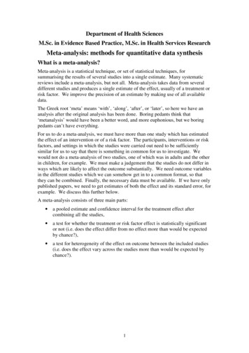
Figure 4. Rates of Caesarean section in trials of nulliparous women receivingepidural analgesia or parenteral opioids Liu EHC and Sia ATH. (2004)RR, natural scale123PooledStudy numberRatio of percentage healed.512 3 4Ratio of percentage healed0 1 2 3 4Figure 5. Forest plots for risk ratio and odds ratio on the natural and logarithmicscales (data of Fletcher et al., 1997)123PooledStudy numberOR, logarithmic scaleOdds ratio, healed.5 15 10Odds ratio, healed0 2 4 6 8 10OR, natural scaleRR, logarithmic scale123PooledStudy number1823PooledStudy number
For both relative risk and odds ratio we find the standard error of the log ratio ratherthan the ratio. The log ratio also tends to have a Normal distribution. On thelogarithmic scale, confidence intervals are symmetrical. Figure 4 shows a forest plotusing odds ratios rather than relative risks. One small trial has such a large odds ratiowith a very wide interval ands is off the scale, its presence merely indicated by anarrow. If they had wanted to include this confidence interval the rest of theinformation would have squeezed into a very narrow area of the graph, making itdifficult to read.Figure 5 shows forest plots on the natural and logarithmic scales for risk ratio andodds ratio for the venous ulcer trial data. The confidence intervals are asymmetricalon the natural scales, symmetrical on the logarithmic scales.Continuous outcome variablesThere are two main measures of treatment or other effect for a continuous outcomevariable, weighted mean difference and standardised mean difference.The weighted mean difference takes the difference in effect, measured in the units ofthe original variable, and weights them by the variance of the estimate. It is in thesame units as the observations, which makes it easy to interpret. It is useful when theoutcome is always the same measurement. These are usually physical measurements.For example, Figure 6 shows the results of a meta-analysis where the outcomevariable is blood pressure measured in mm Hg.The standardised mean difference is found by turning the individual study effectestimates into standard deviation units. We divide the estimate by the standarddeviation of the measurement, either using the common standard deviation withingroups for the study, as found in a two-sample t test, or the standard deviation in thecontrol group. This is also called the effect size. We also divide the standard error ofthe difference by this standard deviation. We then find the weighted average asabove. This is useful when the outcome is not always the same measurement. It isoften used for psychological scales. Figure 7 shows an example of the use ofstandardised mean difference, the outcome variables being various pain scales used tomeasure the outcome of trials of non-steroidal anti-inflammatory drugs.The data required for meta-analysis of a continuous outcome variable are, for eachstudy, the difference between means and its standard error. If these are not given inthe paper, provided we have the mean, standard deviation, and sample size for eachgroup, we then find the difference between means and its standard error in the usualway. For standardised differences, we need either the standardised difference and itsstandard error or the standard deviation. In the latter case we can divide thedifference between means by the standard deviation. Everything is then in the sameunits, i.e. standard deviation units.9
Figure 6. Example of weighted mean difference: blood pressure control by homemonitoring (Cappuccio et al., 2004)Figure 7. Example of standardised mean difference: pain scales used to measure theoutcome of trials of non-steroidal anti-inflammatory drugs in osteoarthritic knee pain(Bjordal et al., 2004)10
Unfortunately, the required data are not always available for all published studies.Studies sometimes report different measure of variation. These might be: standard errors confidence intervals reference ranges interquartile ranges range significance test P value ‘Not significant’ or ‘P 0.05’.We need to extracting the information required from what is available. standard errors — this is straightforward, as we know the formula for thestandard error and so provided we have the sample sizes we can calculatestandard deviation, confidence intervals — this is also straightforward, as we can work back to thestandard error, reference ranges — again straightforward, as the reference range is fourstanard deviations wide, interquartile ranges — here we need an assumption about distribution;provided this is Normal we know how many standard deviations wide the IQRshould be, but of course this is often not the case, range — this is very difficult, as not only to we need to make an assumptionabout the distribution but the estimates are unstable and affected by outliers, significance test — sometimes we can work back from a t value to thestandard error, but not from some other tests, such as the Mann Whitney Utest, P value — if we have a t test we can work back to a t value hence to thestandard error, but not for other tests, and we need the exact P value. ‘Not significant’ or ‘P 0.05’ — this is hopeless.11
Figure 8. Example of time to event data: time to visual field loss or deterioration ofoptic disc, or both, among patients randomised to pressure lowering treatment v notreatment in ocular hypertension (Maier et al., 2005)Figure 10. Survival curves for time to death and time to death or admission tohospital in the ExTraMATCH study (ExTraMATCH Collaborative 2004)12
Figure 11. Results of a meta-analysis of trials of exercise training in patients withchronic heart failure, time to death (ExTraMATCH Collaborative 2004)13
Time to event outcome variablesTime-to-event data arise whenever we have subjects followed over time until someevent takes place. Such data are often called survival data, because the earlyapplications were often in time to death. These techniques are also used for time torecurrence of disease, time to discharge from hospital, time to readmission to hospital,time to conception, time to fracture, etc. The usual problem with such data is that notall subjects have an event, so we know only that they were observed to be event-freeup to some point, but not beyond it. Also, usually some of those observed not to havean event were observed for a shorter time than some of those who did have an event.A special body of statistical techniques, survival analysis, have been developed forsuch data.The main effect measure is the hazard ratio. This is the standard outcome measure insurvival analysis. It is the ratio of the risk of having an event at any given time in onegroup divided by the risk of an event in the other.For example, Maier et al. (2005) analysed the time to visual field loss or deteriorationof the optic disc, or both, in patients with ocular hypertension (Figure 9). The patientswere randomised to pressure lowering treatment or to no treatment. A hazard ratiowhich is equal to one represents no difference between the groups. The hazard ratio isactive treatment divided by no treatment, so if the hazard ratio is less than one, thismeans that the risk of visual field loss is less for patients given pressure loweringtreatment. As for risk ratios and odds ratios, hazard ratios are analysed by taking thelog and the results are shown on a logarithmic scale.Individual patient data meta-analysisIn this kind of meta-analysis, we get the raw data from each study. We may thencombine them into a single data set and analyse them like a single, multicentreclinical trial. Alternatively, we may use the individual data to extract thecorresponding summary statistics from each study then proceed as we would usingsummary statistics from published reports.An example was the ExTraMATCH study (ExTraMATCH Collaborative 2004), ameta-analysis of trials of exercise training in patients with chronic heart failure. Ninetrials identified and principal investigators provided a minimum data set in electronicform. Because in this study the trials were pooled to form one data set, individualstudy results are not given. The outcome was time to death or time to death oradmission to hospital. Figure 10 shows the Kaplan Meier survival curves for theexercise and control groups, pooled across the studies. The Kaplan Meier survivalcurve shows the estimated proportion of subjects who have not yet experienced theevent at each time.Figure 11 shows more results from the ExTraMATCH study. This looks like a forestplot as in Figures 1-9, But it is different. It shows the estimated treatment effect forthe subjects as they are grouped by different prognostic variables. It is to show thatthe effects of treatments are not explained by differences in prognostic variablesbetween the groups, highly unlikely in these randomised trials, and also to suggestwhere there might be interactions between treatment and prognostic variables.And finally . . .Meta-analysis is straightforward if the data are straightforward and all available.14
It depends crucially on the data quality and the completeness of the studyascertainment.Martin Bland16 February 2006ReferencesBjordal JM, Ljunggren AE, Klovning A, Slørdal L. (2004) Non-steroidal antiinflammatory drugs, including cyclo-oxygenase-2 inhibitors, in osteoarthritic kneepain: meta-analysis of randomised placebo controlled trials. BMJ, 329, 1317.Cappuccio FP, Kerry SM, Forbes L, Donald A. (2004) Blood pressure control byhome monitoring: meta-analysis of randomised trials. British Medical Journal, 329,145.Chang JT, Morton SC, Rubenstein LZ, Mojica WA, Maglione M, Suttorp MJ, RothEA, Shekelle PG. (2004) Interventions for the prevention of falls in older adults:systematic review and meta-analysis of randomised clinical trials. British MedicalJournal, 328: 680-3.Colman I, Brown MD, Innes GD, Grafstein E, Roberts TE, Rowe BH. (2004)Parenteral metoclopramide for acute migraine: meta-analysis of randomisedcontrolled trials. British Medical Journal, 329, 1369.Etminan M, Takkouche B, Isorna FC, Samii A. (2005) Risk of ischaemic stroke inpeople with migraine: systematic review and meta-analysis of observational studies.British Medical Journal, 330, 63.ExTraMATCH Collaborative. (2004) Exercise training meta-analysis of trials inpatients with chronic heart failure (ExTraMATCH). British Medical Journal, 328,189.Fletcher A, Nicky Cullum N, Sheldon TA. (1997) A systematic review ofcompression treatment for venous leg ulcers. British Medical Journal, 315, 576-580.Liu EHC and Sia ATH. (2004) Rates of caesarean section and instrumental vaginaldelivery in nulliparous women after low concentration epidural infusions or opioidanalgesia: systematic review. British Medical Journal, 328, 1410-12.Maier PC, Funk J, Schwarzer G, Antes G, Falck-Ytter YT. (2005) Treatment ofocular hypertension and open angle glaucoma: meta-analysis of randomisedcontrolled trials. British Medical Journal, 331, 134.15
effect, and then sum them. This gives a chi-squared test with degrees of freedom number of studies - 1. In the metoclopramide trials in Figure 2, the test for heterogeneity gives 2 4.91, df 2, P 0.086. If there is significant heterogeneity, then we have evidence that there are differences between the studies.