WIXLIB

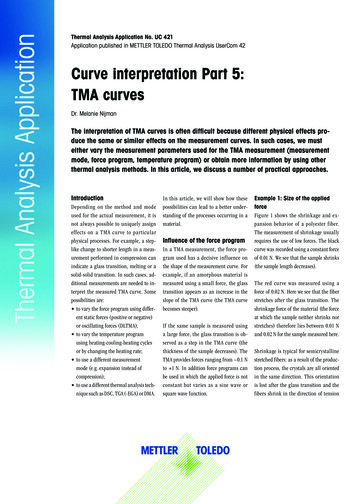
Thermal Analysis ApplicationThermal Analysis Application No. UC 421Application published in METTLER TOLEDO Thermal Analysis UserCom 42Curve interpretation Part 5:TMA curvesDr. Melanie NijmanThe interpretation of TMA curves is often difficult because different physical effects produce the same or similar effects on the measurement curves. In such cases, we musteither vary the measurement parameters used for the TMA measurement (measurementmode, force program, temperature program) or obtain more information by using otherthermal analysis methods. In this article, we discuss a number of practical approaches.IntroductionDepending on the method and modeused for the actual measurement, it isnot always possible to uniquely assigneffects on a TMA curve to particularphysical processes. For example, a steplike change to shorter length in a measurement performed in compression canindicate a glass transition, melting or asolid-solid transition. In such cases, additional measurements are needed to interpret the measured TMA curve. Somepossibilities are: to vary the force program using different static forces (positive or negative)or oscillating forces (DLTMA); to vary the temperature programusing heating-cooling-heating cyclesor by changing the heating rate; to use a different measurementmode (e.g. expansion instead ofcompression); to use a different thermal analysis technique such as DSC, TGA (-EGA) or DMA.In this article, we will show how thesepossibilities can lead to a better understanding of the processes occurring in amaterial.Influence of the force programIn a TMA measurement, the force program used has a decisive influence onthe shape of the measurement curve. Forexample, if an amorphous material ismeasured using a small force, the glasstransition appears as an increase in theslope of the TMA curve (the TMA curvebecomes steeper).If the same sample is measured usinga large force, the glass transition is observed as a step in the TMA curve (thethickness of the sample decreases). TheTMA provides forces ranging from –0.1 Nto 1 N. In addition force programs canbe used in which the applied force is notconstant but varies as a sine wave orsquare wave function.Example 1: Size of the appliedforceFigure 1 shows the shrinkage and expansion behavior of a polyester fiber.The measurement of shrinkage usuallyrequires the use of low forces. The blackcurve was recorded using a constant forceof 0.01 N. We see that the sample shrinks(the sample length decreases).The red curve was measured using aforce of 0.02 N. Here we see that the fiberstretches after the glass transition. Theshrinkage force of the material (the forceat which the sample neither shrinks norstretches) therefore lies between 0.01 Nand 0.02 N for the sample measured here.Shrinkage is typical for semicrystallinestretched fibers: as a result of the production process, the crystals are all orientedin the same direction. This orientationis lost after the glass transition and thefibers shrink in the direction of tension

Thermal Analysis Application(and become thicker). Comparison ofmaterials in this way allows conclusionsto be drawn about differences in production and about the materials themselves.Example 2: DLTMAIn Dynamic Load TMA or DLTMA, theforce acting on the sample varies. We canuse either a sine wave or a square waveforce program. In the square wave forceprogram, the applied force changes periodically from a smaller to a larger value.The values of the two forces and the period (the default value is 12 s) have to bespecified in the method.In the sine wave force program, the applied force varies as a sine function between two forces that also have to be specified in the method. In this case, the periodcan also be freely chosen. Figure 2 showsthe result of a DLTMA measurement of athin 0.5-mm polyethylene terephthalate(PET) disk. For comparison, the curve inthe upper diagram shows the TMA measurement of the same material performedin compression using a constant force.Figure 1. Semicrystalline polyester fiber measured in the tension mode using forces of0.01 N and 0.02 N.The TMA curve shows three clear stepsin which the thickness of the sample decreases as the measurement probe penetrates more and more into the sample.The measurement does not however allow us to unambiguously assign the threeeffects - they could be due to a glass transition, melting, crystallization, shrinkage, decomposition, or other effects.The DLTMA experiment provides us withthe information we need to interpret theTMA measurement curve [1]. Up untilabout 70 C, the change in force has noeffect and the material is hard. At about70 C, the sample softens and the displacement amplitude increases. At thesame time, the material expands andthere is a sudden change in the coefficient of thermal expansion (CTE).Figure 2. Thin PET disk measured using a constant force (0.5 N, above) and an alternatingforce (DLTMA, 0.01 N/ 0.19 N, below).This behavior is typical for a glass transition. The amplitude then decreases, thematerial becomes harder and shrinks.The behavior is characteristic for coldcrystallization. After this transition, thedisplacement amplitude is almost zeroand the material is now hard again butcrystalline and no longer amorphous.Now that we have assigned the first twosteps, the final step can only be due tothe melting of crystallites formed.Example 3: DLTMA with positiveand negative forcesDLTMA measurements are usually performed using positive forces. Certain applications however need alternating positive and negative forces.An example of this is shown in Figure 3,which displays measurement curves ofan initially liquid adhesive. The adhesivewas contained in a 40-µL aluminum cru-METTLER TOLEDOTA Application No. UC 4212

Thermal Analysis Applicationcible to prevent it flowing. The measurement was performed using a flat measurement probe (surface area 1 mm2) at aconstant temperature of 10 C.The force program is shown in the upperright corner of the diagram. The DLTMAcurve (black) initially shows very largedeflections. As long as the sample isliquid, the negative force lifts the probecompletely out of the liquid.After a certain time, with increasingcrosslinking, the viscosity of the adhesive increases and the adhesive becomesincreasingly sticky. As a result of this, thenegative force is no longer sufficient tolift the probe out of the adhesive massand the displacement amplitude becomessmaller until it is almost zero after about40 minutes.The time up to the point when the displacement amplitude first begins to decrease is known as the gel time. This isusually evaluated as the onset of the stepin the envelope difference curve of theupper and lower envelopes.Figure 3. Curing process of an adhesive measured by DLTMA.sine-shaped force excitation is an important measurement parameter whichcan be used to distinguish frequencydependent from frequency-independenteffects. For example, melting alwaysoccurs at the same temperature and isindependent of the frequency. The glasstransition temperature, however, dependson the frequency and shifts to highertemperatures at higher frequencies. Thefrequency dependence of an effect canbest be seen by comparing the modulus curves. The modulus curve can becalculated from the measured DLTMAcurve using the sample geometry and theapplied force program [2].This is illustrated in Figure 4. The upper part of the diagram displays DLTMAcurves of a printed circuit board. Thecurves were recorded using a sine waveforce program with periods of 100 s orThe gel time is the time up until thepoint when an adhesive or a resin systembecomes highly viscous. Terms used inpractical usage are the pot life and working life. All three terms are related butdefined in slightly different ways.Essentially they indicate the period inwhich an adhesive or thermosettingsystem can still be used for its intendedpurpose before it gels or begins to cureand can no longer produce an acceptableresult.Example 4: Influence of frequencyin DLTMA measurementsWhen DLTMA measurements are performed using a sine function force program, the frequency or period of theFigure 4. DLTMA curves of a printed circuit board showing the frequency dependence of theglass transition temperature.METTLER TOLEDOTA Application No. UC 4213

Thermal Analysis Application0.01 Hz (black curve) and 10 s or 0.1 Hz(red curve).The amplitude of the force was 0.48 N.The lower part of the diagram displaysthe corresponding modulus curves. Comparison of the two curves shows thatthe glass transition at the higher frequency is shifted by about 5 K to highertemperature.A simple rule of thumb for the frequencydependence of the glass transition is thatthe glass transition shifts 5 K per decade. A similar rule of thumb also appliesfor DSC measurements: if the heating(or cooling rate) is changed by an orderof magnitude, the glass transition alsoshifts by about 5 K.Temperature programs usingheating–cooling–heatingIn thermal analysis, the so-called thermal history of a sample plays an important role. The thermal history of a sample includes the processing conditions inproduction and the conditions a materialwas exposed to during storage or use. Thethermal history can only be observed inthe first heating run.It is also the reason why the measurement curves of the first and second heating runs are often different. In manycases, it is therefore advisable to measure both the first and the second heatingruns. This applies to TMA, and to DSCand DMA measurements.The example in Figure 5 shows the firstand second heating runs of a PET fibermeasured by DLTMA [3]. In the firstheating run (black curve), the length ofthe fiber remains constant up to about80 C and the displacement amplitudeis small. The fiber then begins to shrinkabove 80 C. At the same time, the fibersoftens and the displacement amplitudeincreases. This behavior is characteristicfor the glass transition of a stretched fiber.Figure 5. First and second heating runs of a PET fiber measured by DLTMA.After the first heating run, all the internal stresses frozen into the fiber duringthe production process have been eliminated through relaxation. As a result, thesample no longer shrinks in the secondheating run.The use of other techniquesSometimes, the properties of a material cannot be clearly characterized byTMA even after varying the force or temperature program. In such cases, otherthermal analysis techniques can providevaluable information and thereby con-tribute to a better understanding of thematerial properties. In the following sections we will discuss different examples.TMA and DSC, and SDTAThe curves colored black in the upperpart of Figure 6 show the TMA curve andpart of the DLTMA curve of a hot melt adhesive [5]. The TMA curve indicates transitions at –37 C and 0 C.These are interpreted as a glass transition and the gel point. The gel point canbe much more easily seen in the DLTMAFigure 6. TMA, DLTMA and DSC measurements of a hot melt adhesive.METTLER TOLEDOTA Application No. UC 4214