WIXLIB

Determinants of rural poverty in UgandaPast research has identified geographical, historical, biophysical and economic factors that influence rural poverty in Uganda. The most frequently quoted factorsare natural resources, farming systems, access to markets and infrastructure, andpopulation density. These factors and their relevance are briefly reviewed below,and potential variables or proxies for these factors are presented.Natural resourcesHuman survival depends on natural resources which are turned, by agricultural andindustrial activities, into goods and services for the maintenance of human communities, their welfare and economic development. In agriculture-dependent subsistence communities, poverty levels are likely to depend on a number of factors thatcan affect agricultural productivity, including; Climate variables, such as temperature and rainfall. Length of the growing period (LGP). Vegetation activity and phenology indicators, such as multi-temporal vegetation indices. Terrain characteristics, such as slope and elevation. Soil quality indicators, such as measures of physical and chemical soil properties.These factors can act and interact in complex ways. For example, acid soils, arefavourable for coffee production but not for maize and bean production. Abundantrainfall can promote crop growth and high yields, but may also favour crop pests.Poor human nutrition leads to lower levels of human health, affecting future productivity.Farming systemsAgricultural activities are the largest source of income in rural Uganda. Greaterlevels of crop and livestock production and greater ownership of land and livestockassets usually suggest greater levels of affluence. A predominance of livestock, however, can also occur in poor communities where livestock is the only livelihoodoption. For example, poor pastoralists are isolated and live a nomadic existence thatis heavily dependent on ruminant livestock. Ownership of mainly monogastric species in a land-less peri-urban context is not indicative of wealth but a reflection ofpoverty. Since this study focuses on livestock production systems, possible relevantvariables from agricultural census data include the densities of cattle, sheep, goats,pigs and poultry. Ideally, however, data on livestock ownership and the contribution made by livestock to peoples’ livelihoods should also be included.Access to markets and infrastructureVon Thünen was a nineteenth century economist and landowner in North Germany who developed a theory of land-use patterns based on the marginal productivity of land at different distances from a major city in which (it was assumed) allthe productivity was sold. In this theory, different types of agricultural productionsystems would be most profitable at different distances from the city (e.g. dairying3

Poverty mapping in Ugandaand intensive farming nearest to the city and ranching farthest from it). Von Thünendirectly and indirectly provided theories on pricing, land use intensity, specialisation and economies of scale (Garnick 1990; Chomitz and Gray 1996). Key variablesto take account of these ideas therefore include distances and time taken to travel toroads, centres of population, markets and agricultural inputs such as labour, animalhealth services and feed (in the case of livestock farming).Population densityAreas of high productivity tend to have high population densities. Higher densitiesof people also imply greater labour availability and greater consumer demand. Rural population densities increase in the vicinity of urban areas and close to transportnetworks, and are naturally correlated with access to markets.Health of people, crops and livestockThe prevalence of diseases - in crops, livestock and people - is also key to welfare.Some of this is direct; human health is itself a measure of welfare and dealing withhuman health problems and controlling diseases in crops and livestock are oftenmajor expenses in poor households, for example. Other effects are indirect; humanill-health impacts on agricultural labour productivity, for example. Whilst explicitdata on these issues may not be available at an appropriate scale and resolution forUganda, there are often strong correlations between disease prevalence or vectorabundance and similar environmental variables to those used here (see for examplethe reviews in Hay et al. 2000 and Pfeiffer et al. 2008). These remotely sensed environmental variables thus have the potential to capture much of the variability in thehealth of people, and their crops and livestock.Other factorsMany other factors have been shown to relate to rural poverty and agriculturalproductivity. Land tenure is one of the most important whereby greater land security is thought to lead to greater output and better land management practices.Access to credit (banks, rural credit systems and micro credit) can make a differenceif directed at small holders, as can the provision of extension services, adoption ofnew products and technology and the capacity to innovate. Unfortunately, suchvariables were not available for Uganda in sufficient detail for their inclusion in thepresent analysis. Here, the emphasis is on remotely sensed and other environmental datasets to provide independent variables for the analyses, resulting in a strongenvironmental bias, as opposed to the more prevalent socio-economic approaches.4

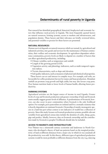
DataThis section describes briefly the data used in the present analysis. Unless otherwisestated, all spatial data are stored as ESRI shape files (points, lines and polygons) orESRI grids (raster) in geographical co-ordinates (Uganda straddles the equator, soscale distortions are minimal). Map legends for expenditure are based on decilescomputed from the household level or aggregated (at about 1km) household levelestimates. Grey shading indicates protected areas on the maps.Household survey dataThe Uganda Bureau of Statistics (UBOS) has carried out a number of nationallyrepresentative surveys since 1988 (see Table 1 in Rogers et al. 2006). In this analysisthe second Uganda National Household Survey (UNHS-2) was used, which wascarried out between May 2002 and April 2003 (UBOS 2003). Data for 5 614 ruralhouseholds with reliable geographical coordinate data were selected from a totalof 9 711 records (urban and rural) in the survey. The dependent variable used wasmonthly household expenditure, corrected for the number of adult equivalents perhousehold. Figure 1 shows the location of the households and Table 1 providessummary statistics for the regional differences in rural per-adult equivalent monthly expenditure in Ugandan Shillings. The monthly expenditure data did not exhibita normal distribution so were transformed before prior to the analysis, as describedbelow.Figure 1. Rural household locations from the 2002-3003 Uganda National Household survey, showing monthly adult equivalent expenditure (in Uganda shillings).NorthernEasternCentralWesternMonthly ependiture 2 900 - 11 800 11 800 - 15 200 15 200 - 18 300 18 300 - 21 400 21 400 - 24 800 24 800 - 28 900 28 900 - 33 900 33 900 - 42 100 42 100 - 59 000 59 000 - 864 500Note: The administrative boundaries shown refer to the four regions of the country.5

Poverty mapping in UgandaThere are clear regional differences, with the Central and Western regions havinghigher levels of expenditure and correspondingly lower percentages of householdsbelow the poverty line than the Eastern and Northern regions. Across Uganda, 38percent of the rural households in the survey were below the poverty line, but thisvaries from 24 percent in the Central region to 60 percent in the Northern region.Table 1. Descriptive statistics for rural, monthly adult equivalent expenditure2002-2003.a) Summary statisticsRegionCountMeanStd Err MeanStd DevSkewnessKurtosisUganda5 61432 49241731 2557.6130.2Central1 51541 1531 00939 2868.1135.4Western1 47934 23771127 3323.622.8Eastern1 56328 81375429 8169.0131.5Northern1 05723 07461419 9624.845.0b) Quartiles including the Inter Quartile Range (Upper – Lower Quartile)RegionMinimumLwr QMedianUpr QMaximumIQ RangeUganda2 91516 72824 81337 377864 53420 649Central4 75221 85831 14047 200864 53425 342Western3 55618 38226 91040 002349 20021 620Eastern4 44415 59522 68132 809608 58917 215Northern2 91512 10218 13826 722304 40014 620c) Poverty lines and ratesRegionPoverty lineAboveBelowAbove %Below %Uganda20 7603 4662 14862%38%Central21 3221 15635976%24%Western20 3081 01046968%32%Eastern20 65287568856%44%Northern20 87242563240%60%Small Area Estimate poverty dataWhilst various methods have been used for poverty mapping, some reviewed byDavis (2003), the most common is the SAE technique, discussed by Ghosh andRao (1994) and developed and exemplified in a series of World Bank studies (e.g.Hentschel et al. 2000; Elbers and Lanjouw 2000; World Bank 2000). This involvesthe application of econometric techniques to combine sample survey data with census data to predict poverty indicators using all households covered by the census.The survey provides the specific poverty indicator and the parameters, based onregression models, to predict the poverty levels for the census households. Usuallythe poverty indicator is a consumption- or expenditure-based indicator of welfare,such as the proportion of households that fall below a certain expenditure level(i.e. the poverty line). The basic methodology is quite simple. At the ‘zero stage’the comparability of data sources is established and variables common to the census and survey are identified. In the ‘first stage’ a regression model is estimated6

Databetween log per capita consumption or expenditure in the household survey andthe variables common both to survey and census. The model thus provides a set ofempirical regression parameters. These regressions are generally nested at variousspatial levels, from regional down to household levels. In the ‘second stage’ theseregression parameters are applied to the census households, where they are used topredict consumption or expenditure in the much more extensive census population, and thus to estimate poverty and inequality for each group of interest. Theprecision of the poverty estimates is evaluated by computing standard errors, whichincrease with the level of disaggregation. In general:y i Ai′β i ε iwhere yi is the welfare indicator for household i, Ai′ is a vector of independent variables (and associated parameters, βi) common to the welfare survey and the censusand εi is a normally distributed error term.Small area poverty estimates have been made for a number of countries, for example Ecuador (Hentschel et al. 2000), South Africa (Alderman et al. 2000; Statistics South Africa 2000), Nicaragua (Arcia et al. 1996); Vietnam (Minot et al. 2003);Epprecht and Heinimann 2004); Kenya (Ndeng’e et al. 2003); and Uganda (Emwanu et al. 2003; 2007).At the time that Rogers et al. (2006) published their working paper, small areaestimates (SAE) of welfare had not been produced for the UNHS-2 household survey data, so direct comparisons with the environmental approach were not possible.Since then, however, SAE poverty mapping has been applied to the same householdsurvey used in the present analysis. Emwanu et al. (2007) combined informationfrom the 2002/03 UNHS-2 (UBOS 2003) and the 2002 Population and HousingCensus (UBOS 2002) to develop poverty maps at district, county and sub-countylevels. The sub-county estimates are shown in Figure 2.Figure 2. Small area (sub-county) estimates of average rural monthly adult equivalent expenditure (in Uganda shillings).NorthernEasternCentralWesternSource: Emwanu et al. (2007).Monthly ependiture 5 000 - 13 000 13 000 - 17 000 17 000 - 20 000 20 000 - 23 000 23 000 - 26 000 26 000 - 29 000 29 000 - 34 000 34 000 - 40 000 40 000 - 53 000 53 000 - 355 0007

household survey data The Uganda Bureau of Statistics (UBOS) has carried out a number of nationally representative surveys since 1988 (see Table 1 in Rogers et al. 2006). In this analysis the second Uganda National Household Survey (UNHS-2) was used, which was carried out between May 2002 and April 2003 (UBOS 2003). Data for 5 614 rural