Transcription
(2022) 15:207Rohlén et al. BMC Research Noteshttps://doi.org/10.1186/s13104-022-06093-1BMC Research NotesOpen AccessRESEARCH NOTEComparison of decomposition algorithmsfor identification of single motor unitsin ultrafast ultrasound image sequences of lowforce voluntary skeletal muscle contractionsRobin Rohlén1* , Jun Yu2 and Christer Grönlund1AbstractObjective: In this study, the aim was to compare the performance of four spatiotemporal decomposition algorithms(stICA, stJADE, stSOBI, and sPCA) and parameters for identifying single motor units in human skeletal muscle undervoluntary isometric contractions in ultrafast ultrasound image sequences as an extension of a previous study. Theperformance was quantified using two measures: (1) the similarity of components’ temporal characteristics againstgold standard needle electromyography recordings and (2) the agreement of detected sets of components betweenthe different algorithms.Results: We found that out of these four algorithms, no algorithm significantly improved the motor unit identification success compared to stICA using spatial information, which was the best together with stSOBI using either spatialor temporal information. Moreover, there was a strong agreement of detected sets of components between thedifferent algorithms. However, stJADE (using temporal information) provided with complementary successful detections. These results suggest that the choice of decomposition algorithm is not critical, but there may be a methodological improvement potential to detect more motor units.Keywords: Ultrafast ultrasound, Concentric needle electromyography, Motor units, Decomposition algorithms, Blindsource separationIntroductionBlind source separation (BSS) separates a set of sources(e.g., hidden signals) from a set of mixtures of the sources(e.g., observed data) without information about thesources and the mixing process [1]. The goal of BSS is tojointly estimate the sources and the mixing process byonly observing the mixture of the sources, which yieldsan ill-posed inverse problem. Many algorithms can solve*Correspondence: robin.rohlen@umu.se1Department of Radiation Sciences, Biomedical Engineering, UmeåUniversity, 901 87 Umeå, SwedenFull list of author information is available at the end of the articlea BSS problem [2–5], and they rely on different temporal, spatial, or spatiotemporal assumptions (different costfunctions).A typical BSS problem is identifying single motorunits (MUs) from, e.g., multichannel data such as surface electromyography (EMG) [6]. The MU comprisesa bundle of muscle fibres innervated by a motoneuron.Through neural activation, it electrically depolarizesthe MU fibres (referred to as a firing instant) and givesrise to a muscle contraction [7, 8]. Studying the MUs’function is essential in, e.g., diagnosing neuromusculardiseases [8], rehabilitation medicine [9], exercise physiology and sports sciences [10]. In previous work, ourgroup applied a BSS algorithm called spatiotemporal The Author(s) 2022. Open Access This article is licensed under a Creative Commons Attribution 4.0 International License, whichpermits use, sharing, adaptation, distribution and reproduction in any medium or format, as long as you give appropriate credit to theoriginal author(s) and the source, provide a link to the Creative Commons licence, and indicate if changes were made. The images orother third party material in this article are included in the article’s Creative Commons licence, unless indicated otherwise in a credit lineto the material. If material is not included in the article’s Creative Commons licence and your intended use is not permitted by statutoryregulation or exceeds the permitted use, you will need to obtain permission directly from the copyright holder. To view a copy of thislicence, visit http:// creat iveco mmons. org/ licen ses/ by/4. 0/. The Creative Commons Public Domain Dedication waiver (http:// creat iveco mmons. org/ publi cdoma in/ zero/1. 0/) applies to the data made available in this article, unless otherwise stated in a credit line to the data.
Rohlén et al. BMC Research Notes(2022) 15:207independent component analysis (stICA) [3] to identify components in ultrafast ultrasound (UUS) imagesequences [11, 12]. Using simulations, we showed thatthe method had high performance [11], but we couldonly identify about one-third of the active MUs in a validation study [12]. However, it’s still unknown whetherthis successful identification rate depends on thatdecomposition algorithm’s properties and cost function(also referred to as an error function that is pre-definedand minimized).This study aimed to compare the performance of different spatiotemporal decomposition algorithms andparameters for identifying single MUs in human skeletalmuscle under low force voluntary isometric contractionsin UUS image sequences as an extension of a previousstudy [12]. The performance was quantified using twomeasures: (1) the similarity of components’ temporalcharacteristics against gold standard needle electromyography recordings and (2) the agreement of detected setsof components between the different algorithms. As aPage 2 of 7performance baseline, we also quantified performancewithout any decomposition.Main textMethodsExperimental procedureWe collected 64 synchronized measurements [12], fromnine healthy subjects (27–45 years old, four men andfive women), from the cross-section of biceps brachii(Fig. 1A). The synchronized measurements were collected using UUS (40 40 mm field of view, 2 kHz framerate) and concentric needle-EMG (38 0.45 mm, 64 kHzsampling rate). The exclusion criteria were subjects withneuromuscular disease, blood disease, and subjects usingblood-thinning drugs. The duration of each measurement was 2 s. Out of the 64 synchronized measurements,we extracted 91 firing patterns of single MUs from the 64EMG datasets, where some datasets included multipleactive MUs (Additional file 1: Table S2). A firing patternis a sequence of firing instants. The subjects performedFig. 1 Framework for MU identification in ultrafast ultrasound (UUS) image sequences was composed of four stages. A The first stage; dataacquisition. Collecting synchronized UUS and concentric needle electromyography (EMG) measurements on the biceps brachii under low forcevoluntary isometric contractions. B The second stage; calculating tissue velocities (based on the UUS radiofrequency signals). C The third stage;data decomposition. We inserted each region-of-interest (ROI, 25 in total) into four different decomposition algorithms (see Table 1) to extract25 spatiotemporal components. D The fourth and final stage; post-processing. We selected one optimal component out of 625 (25 componentsin each of the 25 ROIs) based on its distance to the needle tip ( 10 mm) and maximal agreement to MU firing rate in terms of RoA. The selectedcomponents’ features are then compared between the different decomposition algorithms
Rohlén et al. BMC Research Notes(2022) 15:207Page 3 of 7low force isometric elbow flexion as a physician inserteda needle electrode into the biceps brachii (about 1% ofmaximum voluntary contraction). An additional sectionfile describes the data collection in more detail (Additional file 1: Data collection).Framework for motor unit identification in ultrasound imagesequencesSingle MUs were identified using the frameworkdescribed in Rohlén et al. [12], but we replaced thedecomposition module. See Fig. 1. In short, we used aspatial sub-region of 20 20 mm as the region-of-interest (ROI) with jumps of 5 mm laterally and axially, resulting in 25 partially overlapping sub-regions (Fig. 1C). Foreach ROI, we reduced the data dimension using singularvalue decomposition. A decomposition algorithm is thenapplied to decompose each ROI into 25 spatiotemporalcomponents (Fig. 1C), where we estimated the firing pattern for each component [12]. This procedure resultedin 25 25 625 components from each synchronizeddataset and algorithm. From all these components, weselected one component per synchronized measurement(excluding components 10 mm from the needle) basedon the maximal rate of agreement (RoA) with the firinginstants of the EMG-measured MU (Fig. 1D). For theRoA definition, see below.Decomposition algorithmsThe objective is to recover the latent componentsS from the observed data Y. Here, we focused on theinstantaneous linear model, Y AS, where Y (Y, ,Y) isthe observed data, S (S, ,S) is the latent components,A is the unobserved mixing matrix, m and n are thenumbers of pixels and latent components respectively. The objective is to transform the observed dataY using a linear transformation W A , which denotesthe pseudo-inverse of A. Thus, S WY. In this work,observed data Y is the UUS velocity data that has beenvectorized from 3D (2D over time) to 2D.We chose four algorithms to be evaluated with different parameters focusing on different spatiotemporal features (see Table 1 for an overview). For details ofeach algorithm, we refer to the corresponding articles.The selected decomposition algorithms are: sparse PCA(sPCA) [2], spatiotemporal independent componentanalysis (stICA) [3], spatiotemporal joint approximation diagonalization of eigenmatrices (stJADE) [4],and spatiotemporal second-order blind identification(stSOBI) [13]. sPCA has a parameter λ related to thenumber of non-zero pixels. In contrast, stICA, stJADE,and stSOBI have a weighting α-parameter favouringtemporal or spatial separation [3].The most common general BSS algorithms are thestICA, stJADE, and stSOBI (or its special cases) andhave been used in other BSS comparison studies [14–17]. For example, the Infomax-based approach [18] isa common algorithm identical to the maximum likelihood approach used here [19]. stSOBI [13] is a spatiotemporal extension to SOBI [5], which is an extensionof AMUSE [20] and has been used in previous studies[21, 22]. We chose sPCA (with spatial cost function) tosolve the BSS problem using a completely different penalty/optimization procedure than the other algorithms.Note that dimension reduction is included in sPCA. WeTable 1 A summary of the selected decomposition algorithms and their parametersAlgorithmParameter (λ or α)DomainDescriptionsPCAλ 150SpatialExtension of principal component analysis (PCA) by sparse constraint, i.e., uses L 1 penalty onthe spatial loadings in the optimization procedure. λ denotes the number of non-zero pixels, aparameter equal to 150 and 250 corresponds to territories with 4.3 and 5.6 mm in diameterλ 250stICAstJADEstSOBIα 0.0SpatialTemporalα 0.8Spatiotemporalα 0.0Temporalα 1.0Spatialα 0.5Spatiotemporalα 0.0Temporalα 1.0α 0.5α 1.0Separation by optimizing a joint entropy energy function based on mutual entropy and infomaxwith a kurtosis-based cost function. α 0.8 has been used previously [11, 12], i.e., weighs 0.8 inspatial and 0.2 in temporal separationJoint diagonalization of fourth-order cumulant tensor in separation procedure. A low α weighsmore on temporal ce matrices (fixed number, 12) for joint diagonalization of a set of symmetrizedmultidimensional autocovariances [28, 29]. Similar to stJADE, a low α weighs more on temporalseparationα-parameter weighs spatial- and temporal separation, a λ-parameter relates to the number of non-zero pixelssPCA sparse principal components, stICA spatiotemporal independent component analysis, stJADE spatiotemporal joint approximation diagonalization ofeigenmatrices, and stSOBI spatiotemporal second-order blind identification
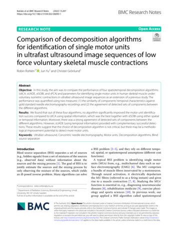
Rohlén et al. BMC Research Notes(2022) 15:207anticipate that all these algorithms, together with theirvarious parameters, should represent a broad spectrumof the instantaneous linear BSS space.We calculated a baseline for the algorithms’ comparison; no decomposition (ND). As with the decompositionalgorithms, we computed mean values in the overlappingROIs of different sizes (20 20 mm, 10 10 mm, and5 5 mm),i.e., ND20, ND10, and ND5. Thus, we com1puted mj Y m, where Y m is the observed data vectorm Rijat pixel m, and Ri denotes a set of indexes in the imagewhere j is ND20, ND10, or ND5 and i is one of the overlapping ROIs. Note that i is of different lengths depending on j due to changing ROI sizes.Performance evaluationThe firing pattern similarity between each componentand MU was calculated using the RoA metric calculatedas RoA 100 cj /(cj Aj Bj ), where cj is the number of firings of the jth firing pattern that was identified, Aj and Bj are the number of false identified firingsand unmatched firings in the jth firing pattern, respectively. The tolerance between each firing of a MU and acomponent was set to 30 ms motivated by the unknownelectromechanical delay [23] and potential noise of thedecomposed component’s causing variation in each estimated component’s firings. We divided RoA of each algorithm into different groups of success, i.e., no-success(0% RoA 50%), semi-success (50% RoA 75%),and high-success (75% RoA 100%). The motivationbehind the thresholds is that 50% RoA is around the peakvalue for “no-decomposition,” and 75% RoA is around theaverage value in the successfully identified RoA group in[12].To determine whether there was a pairwise differencein median RoA between stICA08 and the other decomposition algorithms, we tested the pairwise differencesin median RoA using the two-sided Wilcoxon signedrank test. The stICA08 was used as a reference algorithmbecause it has been used in previous studies [11, 12]. Thep-values were adjusted for multiple testing based on thefalse discovery rate [24].To quantify the agreement of detected sets of components between the different algorithms, we used thecommon id ratio (CIDR) metric that we define as the cardinality of intersection of sets divided by the minimumcardinality in each set where the identified stICA08 MUindices were used as a reference. The CIDR takes a valuebetween 0 and 1, where CIDR 1 means that we foundthe same set of components, and CIDR 0 means thatnone of the detected components of the two methods isequal.Page 4 of 7ResultsPerformance evaluation: firing patternAs a primary analysis, the high-success group is considered, as it relates to the successful one-third [12]. Asecondary analysis relates to the semi-success group.Regarding the primary analysis, stICA08, stICA10,stJADE00, stJADE10, stSOBI00, stSOBI05, and stSOBI10identified 2–9 components (2–10%) with RoA larger than75% (Fig. 2A). There was no pairwise difference in medianRoA between stICA08 and stICA10 (p 0.21), stSOBI00(p 0.17), and stSOBI10 (p 0.07). For all other algorithms, there was a statistically significant difference. NDand sPCA performed the worst, where 91–99% belongedto the no-success group.Regarding the secondary analysis, there was no pairwise difference in median RoA between stICA08 andstICA10 (p 0.26). For all other algorithms, there was astatistically significant difference. See the Additional filefor examples and detailed descriptions (Additional file 1:Fig. S1–S3 and Table S1–S2).Performance evaluation: agreement between detected setsof componentsFor the high-success group, 5 out of 6 algorithms hadCIDR 1.00, whereas stJADE00 had 0.00, meaning itcomplements stICA08 with a different set of components(Fig. 2A). None of the other algorithms did identify thesame components as stJADE00 either (Additional file 1:Table S1). For the semi-success group, the CIDR rangewas 0.38–0.81 (0.58 0.14 , excluding ND and sPCA).stICA10, stJADE and stSOBI found about the same number of components (or more), and they centred at aboutCIDR 0.6 (Fig. 2B), indicating improvement potentialconcerning stICA08. For the no-success group, the CIDRrange was 0.79–0.98 (0.85 0.06, excluding ND andsPCA).DiscussionWe compared the performance of four different spatiotemporal decomposition algorithms and parameter settings for identifying single MUs in UUS image sequencesof skeletal muscle low force voluntary isometric contractions. There are four main findings: (1) Out of thesealgorithms, no algorithm significantly improved the MUidentification success compared to stICA08. (2) stICAwith spatial approach and stSOBI with spatial or temporal approach had the best overall performance. (3) Therewas a strong agreement between different algorithms’identified components. However, there were algorithmswith complementary successful detections. (4) Whenno decomposition method was applied, 96–99% of the
Rohlén et al. BMC Research Notes(2022) 15:207Page 5 of 7Fig. 2 Performance evaluation of the decomposition algorithms (red points) with stICA08 (blue points) as the reference algorithm. The comparisonbetween the algorithms’ performance is based on (1) firing pattern agreement between the components and the EMG reference (RoA), and(2) agreement between the different algorithms’ identified component sets (CIDR). The components’ RoA values were divided into groups; Ahigh-success group (75% RoA 100%), and B semi-success group (50% RoA 75%). Note that the number of components at the x-axis denoteseach algorithm’s number of components within the pre-defined group (high-success or semi-success)components belonged to the no-success group with anaverage agreement below 30%.We found that stICA10 (spatial) and stSOBI00 (temporal) performed similarly in the high-success group.These two algorithms use entirely different cost functions. The former considers sparse territories, and thelatter considers autocorrelated twitch trains, makingsense because they should be sparse and autocorrelated due to the biological nature of the MU and twitch.Interestingly, stSOBI00 and stSOBI10 find the samehigh-RoA components, suggesting that temporal andspatial dependence are robust features for identificationthat could be adapted more explicitly using twitch-likea priori information. stICA00 (temporal) did not haveany component that belonged to the high-success groupsuggesting that the twitch trains are not sparse, whichalso makes sense due to the non-stationary behaviour oftwitches during an unfused tetanic contraction [25, 26].Also, stJADE00 and stJADE10 found a few high-RoAunits. A possible explanation why temporal stJADE00managed to identify high-RoA components, whichstICA00 could not, could be that the joint diagonalization approach is more robust against local minima andnoise [4]. Also, stJADE00 complements the other algorithms with three new high-RoA components that werenot identified by any other algorithm (Fig. 2A).In conclusion, these findings suggest two things.(1) The choice of instantaneous decomposition algorithm is not critical for the present task. (2) There isan improvement potential to optimize the BSS costfunction to detect more MUs in experimental imagesequences of voluntary contracting skeletal muscles.LimitationsWe assumed the firing pattern should be similar inEMG and UUS domains and the electromechanicaldelay was within the tolerance parameter in RoA [12],which is the only way to quantify successful identification in this case. We assumed an instantaneous linearmapping of the mixing matrix. However, a previousstudy suggests that the linear BSS algorithms mayrecover nonlinear mixed sources accurately if the inputdimension is sufficiently higher than the source dimensionality [27].AbbreviationsUUS: Ultrafast ultrasound; MU: Motor unit; BSS: Blind source separation; stICA:Spatiotemporal independent component analysis; stJADE: Spatiotemporaljoint approximation diagonalization of eigenmatrices; stSOBI: Spatiotemporalsecond-order blind identification; sPCA: Sparse principal component analysis;RoA: Rate of agreement; CIDR: Common id ratio; MUAP: Motor unit actionpotential; EMG: Electromyography; ND: No-decomposition; TVI: Tissue velocityimages; ROI: Region of interest.
Rohlén et al. BMC Research Notes(2022) 15:207Supplementary InformationThe online version contains supplementary material available at https:// doi. org/ 10. 1186/ s13104- 022- 06093-1.Additional file 1. A detailed description of the data collection. Figure S1.Pairwise firing pattern rate of agreement (RoA) differences for the threesuccess groups. Figure S2. An example of components’ twitch trainsfor MU #30 regarding three algorithms’ (seven in total considering theirdifferent parameters). Figure S3. The individual rate of agreement (RoA)values for each motor unit (MU) and algorithm. Table S1. Performanceevaluation of decomposition algorithms (in terms of RoA and CIDR).Table S2. The number of MUs extracted from the EMG data per contraction (91/64 1.4 active motor units per measurement/dataset).AcknowledgementsNot applicable.Author contributionsRR and CG designed and performed the experiments; RR and CG performedthe data analysis; and RR, JY, and CG all revised/wrote the paper. All authorsread and approved the final manuscript.Page 6 of 75.6.7.8.9.10.11.12.13.FundingOpen access funding provided by Umeå University. This work was funded bythe Swedish Research Council (Grant Number 2015-04461) and the Kempefoundations (Grant Number JCK-1115).14.Availability of data and materialsThe data supporting this study’s findings are available on request from thecorresponding author RR. The raw data are not publicly available because ofthe large file sizes.15.DeclarationsEthics approval and consent to participateThe subjects gave informed consent verbally and in written form before theexperimental procedure. The project conformed to the Declaration of Helsinkiand was approved by the Swedish Ethical Review Authority (2019-01843).Consent for publicationNot applicable.Competing interestsThe authors declare that they have no competing interests.Author details1Department of Radiation Sciences, Biomedical Engineering, Umeå University,901 87 Umeå, Sweden. 2 Department of Mathematics and Mathematical Statistics, Umeå University, 901 87 Umeå, Sweden.16.17.18.19.20.21.22.23.Received: 8 February 2022 Accepted: 3 June 202224.References1. Hyvärinen A, Karhunen J, Oja E. Independent component analysis. NewYork: Wiley; 2001.2. Zou H, Hastie T, Tibshirani R. Sparse principal component analysis. J Comput Graph Stat. 2006;15:265–86.3. Stone JV, Porrill J, Porter NR, Wilkinson ID. Spatiotemporal independentcomponent analysis of event-related fMRI data using skewed probabilitydensity functions. Neuroimage. 2002;15:407–21.4. Theis FJ, Gruber P, Keck IR, Meyer-Bäse A, Lang EW, Spatiotemporal blindsource separation using double-sided approximate joint diagonalization.In,. 13th European Signal Processing Conference. IEEE. 2005;2005:1–4.25.26.27.Belouchrani A, Abed-Meraim K, Cardoso JF, Moulines E. Second-orderblind separation of temporally correlated sources. In: Proc int conf digitalsignal processing. Princeton: Citeseer; 1993. p. 346–51.Farina D, Holobar A. Characterization of human motor units from surfaceEMG decomposition. Proc IEEE. 2016;104:353–73.Basmajian JV, de Luca CJ. Muscles alive: their functions revealed by electromyography. Philadelphia: Williams and Wilkins; 1985.Preston DC, Shapiro BE. Electromyography and neuromuscular disorders.Philadelphia: Saunders; 2012.Merletti R, Botter A, Cescon C, Minetto MA, Vieira TMM. Advances insurface EMG: recent progress in clinical research applications. Crit RevBiomed Eng. 2010;38:347–79.Türker H, Sözen H. Surface electromyography in sports and exercise. In:Turker H, editor. Electrodiagnosis in new frontiers of clinical research.London: In Tech; 2013.Rohlen R, Stalberg E, Stoverud KH, Yu J, Gronlund C. A method foridentification of mechanical response of motor units in skeletal musclevoluntary contractions using ultrafast ultrasound imaging—simulationsand experimental tests. IEEE Access. 2020;8:50299–311.Rohlén R, Stålberg E, Grönlund C. Identification of single motor units inskeletal muscle under low force isometric voluntary contractions usingultrafast ultrasound. Sci Rep. 2020;10:1–11.Theis FJ, Gruber P, Keck IR, Tomé AM, Lang E. A spatiotemporal secondorder algorithm for fMRI data analysis. In: Proceedings of the secondinternational conference on computational intelligence in medicineand healthcare (CIMED 2005). Lisbon, Portugal: IEEE; 2005. p. 194–201,ISBN:0863415202.Zavala-Fernández H, Sander TH, Burghoff M, Orglmeister R, Trahms L.Comparison of ICA algorithms for the isolation of biological artifacts inmagnetoencephalography. In: international conference on independent component analysis and signal separation. Berlin: Springer; 2006. p.511–8.Klemm M, Haueisen J, Ivanova G. Independent component analysis:comparison of algorithms for the investigation of surface electrical brainactivity. Med Biol Eng Comput. 2009;47:413–23.Naik GR. A comparison of ICA algorithms in surface EMG signal processing. Int J Biomed Eng Technol. 2011;6:363–74.Turnip A. Comparison of ICA-based JADE and SOBI methods EOG artifactsremoval. J Med Bioeng. 2015;4:436–40.Bell AJ, Sejnowski TJ. An information-maximization approach to blindseparation and blind deconvolution. Neural Comput. 1995;7:1129–59.Cardoso J-F. Infomax and maximum likelihood for blind source separation. IEEE Signal Process Lett. 1997;4:112–4.Tong L, Soon VC, Huang YF, Liu R. AMUSE: a new blind identificationalgorithm. In: IEEE international symposium on circuits and systems. NewYork: IEEE; 1990. p. 1784–7.Cichocki A, Shishkin SL, Musha T, Leonowicz Z, Asada T, Kurachi T. EEGfiltering based on blind source separation (BSS) for early detection ofAlzheimer’s disease. Clin Neurophysiol. 2005;116:729–37.Najafabadi FS, Zahedi E, Ali MAM. Fetal heart rate monitoring based onindependent component analysis. Comput Biol Med. 2006;36:241–52.Begovic H, Zhou G-Q, Li T, Wang Y, Zheng Y-P. Detection of the electromechanical delay and its components during voluntary isometric contraction of the quadriceps femoris muscle. Front Physiol. 2014;5:494. https:// doi. org/ 10. 3389/ fphys. 2014. 00494.Benjamini Y, Hochberg Y. Controlling the false discovery rate: a practical and powerful approach to multiple testing. J R Stat Soc Ser B.1995;57:289–300.Raikova R, Celichowski J, Pogrzebna M, Aladjov H, Krutki P. Modeling ofsummation of individual twitches into unfused tetanus for various typesof rat motor units. J Electromyogr Kinesiol. 2007;17:121–30.Raikova R, Pogrzebna M, Drzymała H, Celichowski J, Aladjov H. Variabilityof successive contractions subtracted from unfused tetanus of fast andslow motor units. J Electromyogr Kinesiol. 2008;18:741–51.Isomura T, Toyoizumi T. On the achievability of blind source separationfor high-dimensional nonlinear source mixtures. 2018. https:// doi. org/ 10. 48550/ ARXIV. 1808. 00668.
Rohlén et al. BMC Research Notes(2022) 15:207Page 7 of 728. Cardoso J-F, Souloumiac A. Jacobi angles for simultaneous diagonalization. SIAM J matrix Anal Appl. 1996;17:161–4.29. Yeredor A. Non-orthogonal joint diagonalization in the least-squaressense with application in blind source separation. IEEE Trans signal Process. 2002;50:1545–53.Publisher’s NoteSpringer Nature remains neutral with regard to jurisdictional claims in published maps and institutional affiliations.Ready to submit your research ? Choose BMC and benefit from: fast, convenient online submission thorough peer review by experienced researchers in your field rapid publication on acceptance support for research data, including large and complex data types gold Open Access which fosters wider collaboration and increased citations maximum visibility for your research: over 100M website views per yearAt BMC, research is always in progress.Learn more biomedcentral.com/submissions
decomposition module. See Fig. 1. In short, we used a spatial sub-region of 20 20 mm as the region-of-inter - est (ROI) with jumps of 5 mm laterally and axially, result-ing in 25 partially overlapping sub-regions (Fig. 1C). For each ROI, we reduced the data dimension using singular value decomposition. A decomposition algorithm is then