Transcription
Probabilistic Modelling, Machine Learning,and the Information RevolutionZoubin GhahramaniDepartment of EngineeringUniversity of Cambridge, k/zoubin/MIT CSAIL 2012
An Information Revolution? We are in an era of abundant data:– Society: the web, social networks, mobile networks,government, digital archives– Science: large-scale scientific experiments, biomedicaldata, climate data, scientific literature– Business: e-commerce, electronic trading, advertising,personalisation We need tools for modelling, searching, visualising, andunderstanding large data sets.
Modelling ToolsOur modelling tools should: Faithfully represent uncertainty in our model structureand parameters and noise in our data Be automated and adaptive Exhibit robustness Scale well to large data sets
Probabilistic Modelling A model describes data that one could observe from a system If we use the mathematics of probability theory to express allforms of uncertainty and noise associated with our model. .then inverse probability (i.e. Bayes rule) allows us to inferunknown quantities, adapt our models, make predictions andlearn from data.
Bayes RuleP (hypothesis data) P (data hypothesis)P (hypothesis)P (data)Rev’d Thomas Bayes (1702–1761) Bayes rule tells us how to do inference about hypotheses from data. Learning and prediction can be seen as forms of inference.
How do we build thinking machines?
Representing Beliefs in Artificial IntelligenceConsider a robot. In order to behave intelligentlythe robot should be able to represent beliefs aboutpropositions in the world:“my charging station is at location (x,y,z)”“my rangefinder is malfunctioning”“that stormtrooper is hostile”We want to represent the strength of these beliefs numerically in the brain of therobot, and we want to know what rules (calculus) we should use to manipulatethose beliefs.
Representing Beliefs IILet’s use b(x) to represent the strength of belief in (plausibility of) proposition x.0 b(x) 1b(x) 0x is definitely not trueb(x) 1x is definitely trueb(x y)strength of belief that x is true given that we know y is trueCox Axioms (Desiderata): Strengths of belief (degrees of plausibility) are represented by real numbers Qualitative correspondence with common sense Consistency– If a conclusion can be reasoned in more than one way, then every way shouldlead to the same answer.– The robot always takes into account all relevant evidence.– Equivalent states of knowledge are represented by equivalent plausibilityassignments.Consequence: Belief functions (e.g. b(x), b(x y), b(x, y)) must satisfy the rules ofprobability theory, including Bayes rule.(Cox 1946; Jaynes, 1996; van Horn, 2003)
The Dutch Book TheoremAssume you are willing to accept bets with odds proportional to the strength of yourbeliefs. That is, b(x) 0.9 implies that you will accept a bet: xxis true win 1is false lose 9Then, unless your beliefs satisfy the rules of probability theory, including Bayes rule,there exists a set of simultaneous bets (called a “Dutch Book”) which you arewilling to accept, and for which you are guaranteed to lose money, no matterwhat the outcome.The only way to guard against Dutch Books to to ensure that your beliefs arecoherent: i.e. satisfy the rules of probability.
Bayesian Machine LearningEverything follows from two simple rules:PSum rule:P (x) y P (x, y)Product rule: P (x, y) P (x)P (y x)P (D θ, m)P (θ m)P (θ D, m) P (D m)Prediction:P (D θ, m)P (θ m)P (θ D, m)ZP (x D, m) likelihood of parameters θ in model mprior probability of θposterior of θ given data DP (x θ, D, m)P (θ D, m)dθModel Comparison:P (D m)P (m)P (D)ZP (D m) P (D θ, m)P (θ m) dθP (m D)
Modeling vs toolbox views of Machine Learning Machine Learning seeks to learn models of data: define a space of possiblemodels; learn the parameters and structure of the models from data; makepredictions and decisions Machine Learning is a toolbox of methods for processing data: feed the datainto one of many possible methods; choose methods that have good theoreticalor empirical performance; make predictions and decisions
Bayesian Nonparametrics
Why. Why Bayesian?Simplicity (of the framework) Why nonparametrics?Complexity (of real world phenomena)
Parametric vs Nonparametric Models Parametric models assume some finite set of parameters θ. Given the parameters,future predictions, x, are independent of the observed data, D:P (x θ, D) P (x θ)therefore θ capture everything there is to know about the data. So the complexity of the model is bounded even if the amount of data isunbounded. This makes them not very flexible. Non-parametric models assume that the data distribution cannot be defined interms of such a finite set of parameters. But they can often be defined byassuming an infinite dimensional θ. Usually we think of θ as a function. The amount of information that θ can capture about the data D can grow asthe amount of data grows. This makes them more flexible.
Why nonparametrics? flexibility706050 better predictive performance40302010 more realistic0 10 20024All successful methods in machine learning are essentially nonparametric1: kernel methods / SVM / GP deep networks / large neural networks k-nearest neighbors, .1or highly scalable!6810
Overview of nonparametric models and usesBayesian nonparametrics has many uses.Some modelling goals and examples of associated nonparametric Bayesian models:Modelling goalDistributions on functionsDistributions on distributionsClusteringHierarchical clusteringSparse binary matricesSurvival analysisDistributions on measures.Example processGaussian processDirichlet processPolya TreeChinese restaurant processPitman-Yor processDirichlet diffusion treeKingman’s coalescentIndian buffet processesBeta processesCompletely random measures.
Gaussian and Dirichlet Processes32.521.51f(x) Gaussian processes define a distribution on functions0.50 0.5 1f GP(· µ, c) 1.5 2010203040where µ is the mean function and c is the covariance function.We can think of GPs as “infinite-dimensional” Gaussians Dirichlet processes define a distribution on distributionsG DP(· G0, α)where α 0 is a scaling parameter, and G0 is the base measure.We can think of DPs as “infinite-dimensional” Dirichlet distributions.Note that both f and G are infinite dimensional objects.50x60708090100
Nonlinear regression and Gaussian processesConsider the problem of nonlinear regression:You want to learn a function f with error bars from data D {X, y}yxA Gaussian process defines a distribution over functions p(f ) which can be used forBayesian regression:p(f )p(D f )p(f D) p(D)Let f (f (x1), f (x2), . . . , f (xn)) be an n-dimensional vector of function valuesevaluated at n points xi X . Note, f is a random variable.Definition: p(f ) is a Gaussian process if for any finite subset {x1, . . . , xn} X ,the marginal distribution over that subset p(f ) is multivariate Gaussian.
Gaussian Processes and SVMs
Support Vector Machines and Gaussian ProcessesWe can write the SVM loss as:X1 1min f K f C(1 yifi) f2iX1 1We can write the negative log of a GP likelihood as: f K f ln p(yi fi) c2iEquivalent? No.With Gaussian processes we: Handle uncertainty in unknown function f by averaging, not minimization. Compute p(y 1 x) 6 p(y 1 f̂ , x). Can learn the kernel parameters automatically from data, no matter howflexible we wish to make the kernel. Can learn the regularization parameter C without cross-validation. Can incorporate interpretable noise models and priors over functions, and cansample from prior to get intuitions about the model assumptions. We can combine automatic feature selection with learning using ARD.Easy to use Matlab code: http://www.gaussianprocess.org/gpml/code/
Some ComparisonsTable 1: Test errors and predictive accuracy (smaller is better) for the GP classifier, the supportvector machine, the informative vector machine, and the sparse pseudo-input GP classifier.namesynthcrabsbananaData settrain:test dim250:100080:120400:4900breast-cancer 200:77diabetes468:300flare-solar 860.2284102022342200220062210From (Naish-Guzman and Holden, 2008), using exactly same kernels.linear models. In all cases, we employed the isotropic squared exponential kernel, avoiding here theanisotropic version primarily to allow comparison with the SVM: lacking a probabilistic foundation,its kernel parameters and regularization constant must be set by cross-validation. For the IVM,hyperparameter optimization is interleaved with active set selection as described in [2], while for theother GP models, we fit hyperparameters by gradient ascent on the estimated marginal likelihood,
A ssionClassificationKernelBayesian
OutlineBayesian nonparametrics applied to models of other structured objects: Time Series Sparse Matrices Deep Sparse Graphical Models Hierarchies Covariances Network Structured Regression
Infinite hidden Markov models (iHMMs)Hidden Markov models (HMMs) are widely used sequence models for speech recognition,bioinformatics, text modelling, video monitoring, etc. HMMs can be thought of as time-dependentmixture models.In an HMM with K states, the transitionmatrix has K K elements. Let K .S1S2S3STY1Y2Y3YT 2500word identity200015001000500000.511.522.54word position in textx 10 Introduced in (Beal, Ghahramani and Rasmussen, 2002). Teh, Jordan, Beal and Blei (2005) showed that iHMMs can be derived from hierarchical Dirichletprocesses, and provided a more efficient Gibbs sampler. We have recently derived a much more efficient sampler based on Dynamic Programming(Van Gael, Saatci, Teh, and Ghahramani, 2008). http://mloss.org/software/view/205/ And we have parallel (.NET) and distributed (Hadoop) implementations(Bratieres, Van Gael, Vlachos and Ghahramani, 2010).
Infinite HMM: Changepoint detection and video segmentation(a)(b) (Batting1B00020o0x0inc)gP3000itchi4ng0T00(w/ Tom Stepleton, 2009)e5n0n0i0s
Sparse Matrices
From finite to infinite sparse binary matricesznk 1 means object n has feature k:znk Bernoulli(θk )θk Beta(α/K, 1)α/K FigureNote5:thatP (zmatricesnk 1 α)k ) α/K 1 , so as K grows larger the matrixBinaryand theE(θleft-ordergets sparser. So if Z is N K, the expected number of nonzero entries is N α/(1 α/K) N α. Even in the K limit, the matrix is expected to have a finite number ofnon-zero entries. K results in an Indian buffet process (IBP)
Indian buffet processDishes123456“Many Indian restaurantsin London offer lunchtimebuffets with an apparentlyinfinite number of dishes”7Customers891011121314151617181920 First customer starts at the left of the buffet, and takes a serving from each dish,stopping after a Poisson(α) number of dishes as his plate becomes overburdened. The nth customer moves along the buffet, sampling dishes in proportion totheir popularity, serving himself dish k with probability mk /n, and trying aPoisson(α/n) number of new dishes. The customer-dish matrix, Z, is a draw from the IBP.(w/ Tom Griffiths 2006; 2011)
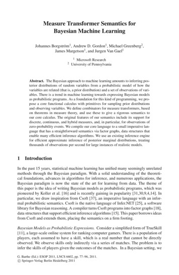
Properties of the Indian buffet processP ([Z] α) exp Y (N mk )!(mk 1)!αK αHN QN!h 0 Kh !k K Prior sample from IBP with α 1001020Shown in (Griffiths and Ghahramani 2006, 2011): It is infinitely exchangeable.The number of ones in each row is Poisson(α)The expected total number of ones is αN .The number of nonzero columns grows as O(α log N ).objects (customers)30405060708090Additional properties:10001020304050features (dishes) Has a stick-breaking representation (Teh, et al 2007) Has as its de Finetti mixing distribution the Beta process (Thibaux and Jordan 2007) More flexible two and three parameter versions exist (w/ Griffiths & Sollich 2007; Tehand Görür 2010)
The Big Picture:Relations between some PifHMMfactorialDPMiHMMtimenon-param.
Modelling Data with Indian Buffet ProcessesLatent variable model: let X be the N D matrix of observed data, and Z be theN K matrix of binary latent featuresP (X, Z α) P (X Z)P (Z α)By combining the IBP with different likelihood functions we can get different kindsof models: Models for graph structures(w/ Wood, Griffiths, 2006; w/ Adams and Wallach, 2010) Models for protein complexes Models for choice behaviour Models for users in collaborative filtering Sparse latent trait, pPCA and ICA models Models for overlapping clusters(w/ Chu, Wild, 2006)(Görür & Rasmussen, 2006)(w/ Meeds, Roweis, Neal, 2007)(w/ Knowles, 2007, 2011)(w/ Heller, 2007)
Nonparametric Binary Matrix Factorizationgenes patientsusers moviesMeeds et al (2007) Modeling Dyadic Data with Binary Latent Factors.
LearningStructureof DeepSparse Graphical ModelsMulti-LayerBeliefNetworks.Zoubin Ghahramani ::Cambridge / CMU ::33
LearningStructureof DeepSparse Graphical ModelsMulti-LayerBeliefNetworks.Zoubin Ghahramani ::Cambridge / CMU ::34
LearningStructureof DeepSparse Graphical ModelsMulti-LayerBeliefNetworks.Zoubin Ghahramani ::Cambridge / CMU ::35
Multi-LayerBeliefNetworksLearningStructureof DeepSparse Graphical Models.ZoubinGhahramani:: HannaCambridge/ CMU:: 36(w/ RyanP. Adams,Wallach,2010)
Learning Structure of Deep Sparse Graphical ModelsOlivettiFaces: 350 Reconstructions50 images of 40 faces (64 &64) FeaturesOlivetti:Inferred: 3 hidden layers, 70 units per layer.Reconstructions and Features:
Olivetti:FantasiesActivationsLearningStructureof Deep&SparseGraphical ModelsFantasies and Activations:Zoubin Ghahramani ::Cambridge / CMU ::47
Hierarchies& % # true hierarchies parameter tying visualisation and interpretability"!
Dirichlet Diffusion Trees (DDT)(Neal, 2001)In a DPM, parameters of one mixture component are independent of othercomponents – this lack of structure is potentially undesirable.A DDT is a generalization of DPMs with hierarchical structure between components.To generate from a DDT, we will consider data points x1, x2, . . . taking a randomwalk according to a Brownian motion Gaussian diffusion process. x1(t) Gaussian diffusion process starting at origin (x1(0) 0) for unit time. x2(t) also starts at the origin and follows x1 but diverges at some time τ , atwhich point the path followed by x2 becomes independent of x1’s path. a(t) is a divergence or hazard function, e.g. a(t) 1/(1 t). For small dt:a(t)dtP (xi diverges at time τ (t, t dt)) mwhere m is the number of previous points that have followed this path. If xi reaches a branch point between two paths, it picks a branch in proportionto the number of points that have followed that path.
Dirichlet Diffusion Trees (DDT)Generating from a DDT:Figure from (Neal 2001)
Pitman-Yor Diffusion TreesGeneralises a DDT, but at a branch point, the probability of following each branchis given by a Pitman-Yor process:bk α,m θθ αKP(diverging) ,m θP(following branch k) to maintain exchangeability the probability of diverging also has to change. naturally extends DDTs (θ α 0) to arbitrary non-binary branching infinitely exchangeable over data prior over structure is the most general Markovian consistent and exchangeabledistribution over trees (McCullagh et al 2008)(w/ Knowles 2011)
Pitman-Yor Diffusion Tree: Results& % Ntrain 200, Ntest 28, D 10 Adams et al. (2008)#"!Figure: Density modeling of the D 10, N 200 macaque skullmeasurement dataset of Adams et al. (2008). Top: Improvement in testpredictive likelihood compared to a kernel density estimate. Bottom:Marginal likelihood of current tree. The shared x-axis is computationtime in seconds.
Covariance Matrices
Covariance Matrices!"# %&'()#*Consider the problem of modelling a covariance matrix Σ that can change as a!"# %&'#'(#)(*" #%#,-.,#*-)"&/-(&% #########0,%&.-&.#0(1%2-%&0"#)%'2-34function of time, Σ(t), or other input variables Σ(x). This is a widely studiedproblem in Econometrics.!!Models commonly used are multivariate GARCH, and multivariate stochasticvolatility models, but these only depend on t, and generally don’t scale well.
Generalised Wishart Processes for Covariance modellingModelling time- and spatially-varying covariancematrices. Note that covariance matrices have tobe symmetric positive (semi-)definite.If ui N , then Σ Pν i 1 ui uiis s.p.d. and has a Wishart distribution.We are going to generalise Wishart distributions to be dependent on time or otherinputs, making a nonparametric Bayesian model based on Gaussian Processes (GPs).So if ui(t) GP, then Σ(t) Pν i 1 ui (t)ui (t)defines a Wishart process.This is the simplest form, many generalisations are possible.Also closely linked to Copula processes.(w/ Andrew Wilson, 2010, 2011)
Generalised Wishart Process Results!"# %&'()*'!"#" %&'()* ,-'./0-'/0-'1.2345(,"'./0'67# 7879: ; ' * ")8 )?6'7 6'9 ? " 7 )6'@7 '1AB': %';7C";7, %D' '67?*;: "%': %'87 : 97:;'%: :-'"E" '7 '; F")'%7?" 67 6@GHD': %' '%: :' ,: '76'"6 "97:;; '6*7 "%' '.2345I'J 'HK'"L*7 '7 %"M'%: :-'*67 #':'./0'F7 ,':'6L*:)"%'"M " 7:;'9 E:)7: 9"'8* 9 7 -'8 )"9:6 '; #';7C";7, %6':)"&'!!!"# ,-./-''''/0&'NONP-'''QBRR'1.2345&'SOTPI'''
Gaussian process regression networksA model for multivariate regression which combines structural properties of Bayesianneural networks with the nonparametric flexibility of Gaussian processesW11 (x)f1 (x)W12 (x)y1 (x)W21 (x)W31 (x)W22 (x)f2 (x)y2 (x)W32 (x)y3 (x)y(x) W (x)[f (x) σf ] σy z(w/ Andrew Wilson, David Knowles, 2011)
Gaussian process regression networks: propertiesW11 (x)f1 (x)W12 (x)y1 (x)W21 (x)W31 (x)W22 (x)f2 (x)y2 (x)W32 (x)y3 (x) multi-output GP with input-dependent correlation structure between the outputs naturally accommodates nonstationarity, heteroskedastic noise, spatially varyinglengthscales, signal amplitudes, etc has a heavy-tailed predictive distribution scales well to high-dimensional outputs by virtue of being a factor model if the input is time, this makes a very flexible stochastic volatility model efficient inference without costly inversions of large matrices using elliptical slicesampling MCMC or variational Bayes
Gaussian process regression networks: resultsGENE (50D)SET 1:GPRN (VB)GPRN (MCMC)LMCCMOGPSLFMSET 2:GPRN (VB)GPRN (MCMC)LMCCMOGPSLFMGENE (1000D)GPRN (VB)GPRN (MCMC)MFITCMPITCMDTCJURAGPRN (VB)GPRN* (VB)SLFM (VB)SLFM* (VB)SLFMCo-krigingICMCMOGPGPAverage SMSEAverage MSLL0.3356 0.02940.3236 0.03110.6909 0.02940.4859 0.03870.6435 0.0657 0.5945 0.0536 0.5523 0.0478 0.2687 0.0594 0.3617 0.0511 0.2376 0.04560.3403 0.03390.3266 0.03210.6194 0.04470.4615 0.06260.6264 0.0610 0.6142 0.0557 0.5683 0.0542 0.2360 0.0696 0.3811 0.0748 0.2528 0.04530.3473 0.00620.4520 0.00790.5469 0.01250.5537 0.01360.5421 0.0085 0.6209 0.0085 0.4712 0.0327 0.3124 0.0200 0.3162 0.0206 0.2493 0.0183Average SMSEAverage MSLLAverage MAETraining Time (secs)0.4040 0.00060.4525 0.00360.4247 0.00040.4679 0.00300.4578 0.00250.510.4608 0.00250.4552 0.00130.5739 0.0003378145601643185079250778474GPEXCHANGEGPRN (VB)GPRN (MCMC)GWPWPMGARCHEmpiricalEQUITYGPRN (VB)GPRN (MCMC)GWPWPMGARCHEmpirical0.5739 0.0003Historical MSE3.83 10 86.120 10 93.88 10 93.88 10 93.96 10 94.14 10 9Historical MSE0.978 10 90.827 10 92.80 10 93.96 10 96.69 10 97.57 10 974L Forecast207320122020195020502006L Forecast274026302930171027602370
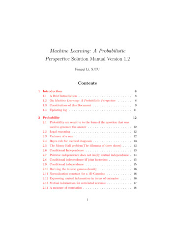
Gaussian process regression networks: 23longitude450.15Predicted correlations between cadmium and zinc
Summary Probabilistic modelling and Bayesian inference are two sides of the same coin Bayesian machine learning treats learning as a probabilistic inference problem Bayesian methods work well when the models are flexible enough to capturerelevant properties of the data This motivates non-parametric Bayesian methods, e.g.:––––––Gaussian processes for regression and classificationInfinite HMMs for time series modellingIndian buffet processes for sparse matrices and latent feature modellingPitman-Yor diffusion trees for hierarchical clusteringWishart processes for covariance modellingGaussian process regression networks for multi-output regression
Thanks toRyan AdamsHarvardTom GriffithsBerkeleyDavid KnowlesCambridgeAndrew nzoubin@eng.cam.ac.uk
Some References Adams, R.P., Wallach, H., Ghahramani, Z. (2010) Learning the Structure of Deep SparseGraphical Models. AISTATS 2010. Griffiths, T.L., and Ghahramani, Z. (2006) Infinite Latent Feature Models and the Indian BuffetProcess. NIPS 18:475–482. Griffiths, T.L., and Ghahramani, Z. (2011) The Indian buffet process: An introduction andreview. Journal of Machine Learning Research 12(Apr):1185–1224. Knowles, D.A. and Ghahramani, Z. (2011) Nonparametric Bayesian Sparse Factor Models withapplication to Gene Expression modelling. Annals of Applied Statistics 5(2B):1534-1552. Knowles, D.A. and Ghahramani, Z. (2011) Pitman-Yor Diffusion Trees. In Uncertainty inArtificial Intelligence (UAI 2011). Meeds, E., Ghahramani, Z., Neal, R. and Roweis, S.T. (2007) Modeling Dyadic Data with BinaryLatent Factors. NIPS 19:978–983. Wilson, A.G., and Ghahramani, Z. (2010, 2011) Generalised Wishart Processes.arXiv:1101.0240v1. and UAI 2011 Wilson, A.G., Knowles, D.A., and Ghahramani, Z. (2011) Gaussian Process Regression Networks.arXiv.
Appendix
Support Vector MachinesConsider soft-margin Support Vector Machines:X12min kwk C(1 yifi) w2iwhere () is the hinge loss and fi f (xi) w · xi w0. Let’s kernelize this:xi φ(xi) k(·, xi),w f (·)By reproducing property:By representer theorem, solution:hk(·, xi), f (·)i f (xi).Xf (x) αik(x, xi)iDefining f (f1, . . . fN )T note that f Kα, so α K 1fTherefore the regularizer 12 kwk2 21 kf k2H 21 hf (·), f (·)iH 12 α Kα 12 f K 1fSo we can rewrite the kernelized SVM loss as:X1 1min f K f C(1 yifi) f2i
Posterior Inference in IBPsP (Z, α X) P (X Z)P (Z α)P (α)Gibbs sampling:P (znk 1 Z (nk), X, α) P (znk 1 Z (nk), α)P (X Z)m n,kN For infinitely many k such that m n,k 0: Metropolis steps with truncation tosample from the number of new features for each object. If α has a Gamma prior then the posterior is also Gamma Gibbs sample. If m n,k 0,P (znk 1 z n,k ) Conjugate sampler: assumes that P (X Z) can be computed.RNon-conjugate sampler: P (X Z) P (X Z, θ)P (θ)dθ cannot be computed,requires sampling latent θ as well (e.g. approximate samplers based on (Neal 2000)non-conjugate DPM samplers).Slice sampler: works for non-conjugate case, is not approximate, and has anadaptive truncation level using an IBP stick-breaking construction (Teh, et al 2007)see also (Adams et al 2010).Deterministic Inference: variational inference (Doshi et al 2009a) parallel inference(Doshi et al 2009b), beam-search MAP (Rai and Daume 2011), power-EP (Ding et al 2010)
Probabilistic Modelling A model describes data that one could observe from a system If we use the mathematics of probability theory to express all . Machine Learning is a toolbox of methods for processing data: feed the data into one of many possible methods; choose methods that have good theoretical or empirical performance; make predictions .