Transcription
STAT/Q SCI 403: Introduction to Resampling MethodsSpring 2017Lecture 5: BootstrapInstructor: Yen-Chi ChenQuestion 1: error of sample median? We start with a simple example: what is the error of samplemedian? Like sample mean is an estimate of the mean of population, the sample median is an estimate ofthe median of population. Because it is an estimator, we can define the bias, variance, and mean squareerror (MSE) of sample median. But what are these quantities?Question 2: confidence interval of sample median? Moreover, how can we construct a confidenceinterval for the population median? We know that given a random sample X1 , · · · , Xn F , a 1 α confidenceinterval of population mean isσbnX̄n z1 α/2 · ,nwhere X̄n and σbn are the sample mean and sample standard deviation. Can we do the same thing (constructa confidence interval) for the median?In this lecture, we will address these problems for median and many other statistics using the well-knownapproach: the bootstrap.5.1Empirical BootstrapHere is how we can estimate the error of sample median and construct the corresponding confidence interval.Assume we are given the data points X1 , · · · , Xn . Let Mn median{X1 , · · · , Xn }. First, we sample with (1) (1)replacement from these n points, leading to a set of new observations denoted as X1 , · · · , Xn . Again,we repeat the sample procedure again, generating a new sample from the original dataset X1 , · · · , Xn by (2) (2)sampling with replacement, leading to another new sets of observations X1 , · · · , Xn . Now we keeprepeating the same process of generating new sets of observations, after B rounds, we will obtain (1), · · · , Xn (1) (2), · · · , Xn (2).X1X1. (B)X1, · · · , Xn (B) . (1) (1)So totally, we will have B sets of data points. Each set of the data points, say X1 , · · · , Xn , is called abootstrap sample. This sampling approach–sample with replacement from the original dataset–is called theempirical bootstrap, invented by Bradley Efron (sometimes this approach is also called Efron’s bootstrap ornonparametric bootstrap)1 .Now for each set of data, we then compute their sample median. This leads to B sample medians, called1 Formore details, check the wikipedia: https://en.wikipedia.org/wiki/Bootstrapping (statistics)5-1
5-2Lecture 5: Bootstrapbootstrap medians: (1), · · · , Xn (1) } (2), · · · , Xn (2) }Mn (1) median{X1Mn (2) median{X1. (B)Mn (B) median{X1, · · · , Xn (B) }.Now here are some real cool things. (1) Bootstrap estimate of the variance. We will use the sample variance of Mnestimate of the variance of sample median Mn . Namely, we will useBdB (Mn ) Var 21 X ( )Mn M̄B ,B 1M̄B 1 (B), · · · , Mnas anB1 X ( )Mn ,B 1as an estimate of Var(Mn ). Bootstrap estimate of the MSE. Moreover, we can estimate the MSE byB 21 X ( )\MSE(Mn ) Mn Mn .B 1 Bootstrap confidence interval. In addition, we can construct a 1 α confidence interval of thepopulation median viaqdB (Mn ).Mn z1 α/2 · VarWell. this sounds a bit weird–we generate new data points by sampling from the existing data points.However, under some conditions, this approach does work! And here is a brief explanation on why thisapproach works.Let X1 , · · · , Xn F . Recall from Lecture 1, a statistic S(X1 , · · · , Xn ) is a function of random variables soits distribution will depend on the CDF F and the sample size n. Thus, the distribution of median Mn ,denoted as FMn , will also be determined by the CDF F and sample size n. Namely, we may write the CDFof median asFMn (x) Ψ(x; F, n),(5.1)where Ψ is some complicated function that depends on CDF of each observation F and the sample size n.bWhenPn we sample with replace from X1 , · · · , Xn , what is the distribution we are sampling from? Let Fn (x) 1I(X thatjumpsateachdataii 1npoint. We know that for a discrete random variable, each jump point in its CDF corresponds to the possiblevalue of this random variable and the size of the jump is the probability of selecting that value.Therefore, if we generate a random variable Z from Fbn , then Z has the following probability distribution:P (Z Xi ) 1,nfor each i 1, 2, · · · , n.If we generated IID Z1 , · · · , Zn Fbn , then the distribution of each Z isP (Z Xi ) 1,nfor each i 1, 2, · · · , n, and for all 1, · · · , n.
Lecture 5: Bootstrap5-3What is this sample Z1 , · · · , Zn ? This sample is a sample generated by sampling with replacement fromX1 , · · · , Xn . (1) (1)Recall that each set of the bootstrap sample, say X1 , · · · , Xn , is obtained via sampling with replacementfrom X1 , · · · , Xn . Thus, each set of the bootstrap sample is an IID sample from Fbn . Namely, (1), · · · , Xn (1) Fbn (2), · · · , Xn (2) Fbn.X1X1 (B)X1 (1)Because a bootstrap median, say Mn(5.1), is, · · · , Xn (B) Fbn . (1), is the sample median of X1 (1), · · · , Xn. Its CDF, by equationFM (1) (x) Ψ(x; Fbn , n).nAnd because each of the bootstrap sample are all from the distribution Fbn , we will haveΨ(x; Fbn , n) FM (1) (x) FM (2) (x) · · · FM (B) (x).nnnWe know that Fbn is very similar to F when the sample size is large. Thus, as long as Ψ is smooth (smoothlychanging) with respect to F , Ψ(x; Fbn , n) will also be very similar to Ψ(x; F, n), i.e.,Fbn F FM ( ) (x) Ψ(x; Fbn , n) Ψ(x; F, n) FMn (x).nThis means:The CDF of a bootstrap median, FM ( ) (x), is approximating the CDF of the true median, FMn (x).nThis has many implications. For an example, when two CDFs are similar, their variances will be similar aswell, i.e., Var Mn ( ) X1 , · · · , Xn Var(Mn ).2dB (Mn ) is just a sample variance of M ( ) . When B is large, theNow the bootstrap variance estimate Varsample variance is about the same as the population variance, implyingBdB (Mn ) Var 2 1 X ( )Mn M̄B Var Mn ( ) X1 , · · · , Xn .B 1 1Therefore, dB (Mn ) Var M ( ) X1 , · · · , Xn Var(Mn ),Varnwhich explains why the bootstrap variance is a good estimate of the true variance of the median.Generalization to other statistics. The bootstrap can be applied to many other statistics such as samplequantiles, interquartile range, skewness (related to E(X 3 )), kurtosis (related to E(X 4 )), .etc. The theorybasically follows from the same idea.2 The reason why in the left-hand-side, the variance is conditioned on X , · · · , X is because when we compute the bootstrapn1estimate, the original observations X1 , · · · , Xn are fixed.
5-4Lecture 5: BootstrapFailure of the bootstrap. However, the bootstrap may fail for some statistics. One example is theminimum value of a distribution. Here is an illustration why the bootstrap fails. Let X1 , · · · , Xn Uni[0, 1]and Mn min{X1 , · · · , Xn } be the minimum value of the sample. Then it is known thatDn · Mn Exp(1). : Think about why it converges to exponential distribution.Thus, Mn has a continuous distribution. Assume we generate a bootstrap sample X1 , · · · , Xn from theoriginal observations. Now let Mn min{X1 , · · · , Xn } be the minimum value of a bootstrap sample.Because each X has an equal probability ( n1 ) of selecting each of X1 , · · · , Xn , this impliesP (X Mn ) 1.nNamely, for each observation in the bootstrap sample, we have a probability of 1/n selecting the minimumvalue of the original sample. Thus, the probability that we do not select Mn in the bootstrap sample is n 1 e 1 .P (none of X1 , · · · , Xn select Mn ) 1 nThis implies that with a probability 1 e 1 , one of the observation in the bootstrap sample will select theminimum value of the original sample Mn . Namely,P (Mn Mn ) 1 e 1 .Thus, Mn has a huge probability mass at the value Mn , meaning that the distribution of Mn will not beclose to an exponential distribution.5.2Parametric BootstrapWhen we assume the data is from a parametric model (e.g., from Normal distribution, exponential distribution, .etc), we can use the parametric bootstrap to access the uncertainty (variance, mean square errors,confidence intervals) of the estimated parameter. Here is an illustration using the variance of a normaldistribution.22Example: normal distribution. Let X1 , · · · , Xn N (0,Pσn ), where σ 2is an unknown number. A natural122way to estimate σ is via the sample variance Sn n 1 i 1 (Xi X̄n ) . Because the sample variance isan estimator, it is a random quantity. How do we estimate the variance of the sample variance? How do weestimate the MSE of the sample variance? How do we construct a 1 α confidence interval for σ 23 ?Here is what we are going to do. Because we know that the sample variance is a good estimator of σ 2 , we canuse it to replace σ 2 , leading to a new distribution N (0, Sn2 ). We know to sample from this new distribution,so we just generate bootstrap samples from this distribution. Assume we generate B sets of samples: (1), · · · , Xn (1) N (0, Sn2 ) (2), · · · , Xn (2) N (0, Sn2 ).X1X1 (B)X13 Some, · · · , Xn (B) N (0, Sn2 ).of you might have learned an approach via inverting the χ2 distribution. That is a viable approach as well.
Lecture 5: Bootstrap5-52 (1)2 (B)To estimate the variability of Sn2 , we use the sample variance of each bootstrap sample. Let Sn , · · · , Sn2 ( ) ( ) ( )be the sample variance of each bootstrap sample (Snis the sample variance of X1 , · · · , Xn ).We then useBdB (S 2 ) Varn 1 X 2 ( )2 ,Sn S̄BB 12 S̄B 1B1 X 2 ( )Sn ,B 1as an estimator of the variance of the original sample variance, i.e., Var(Sn2 ). Similarly, the MSE can beestimated byB 2X[ B (Sn2 ) 1MSESn2 ( ) Sn2 .B 12And a confidence interval of σ can be constructed usingqdB (S 2 ).S 2 z1 α/2 · VarnnThis approach, sampling from the distribution formed by plugging the estimated parameters, is called parametric bootstrap.Example: exponential distribution. The similar approach applies to many other models. For example,if we assume the data X1 , · · · , Xn Exp(λ), where λ is an unknown quantity. And we estimate λ by anbn 1 . To assess the quality of λbn , say the its MSE, we first generate Bestimator such as the MLE λX̄nbootstrap samples: (1)bn ), · · · , Xn (1) Exp(λ (2)bn ), · · · , Xn (2) Exp(λ.X1X1 (B)X1bn )., · · · , Xn (B) Exp(λThen using each sample, we obtain a bootstrap estimate of λ:b (1) , · · · , λb (B) , where λb ( ) λnnn1 ( )X̄n 1 ( )X1 ( ) ··· Xnn.bn can be estimated byThen the MSE of λB 2Xbn ) 1b ( ) λbn .[ B (λλMSEnB 15.3 :Remark on the BootstrapThere are some variants of bootstrap such as the Jackknife4 (leave one observation out each time) andsubsampling (only subsample m out of n sample).Moreover, when the data are dependent such as the time series dataset or spatial dataset, the bootstrap canalso be applied; in these case, one will use the block bootstrap5 or spatial bootstrap.4 https://en.wikipedia.org/wiki/Jackknife resampling5 https://en.wikipedia.org/wiki/Bootstrapping (statistics)#Block bootstrap
5-4 Lecture 5: Bootstrap Failure of the bootstrap. However, the bootstrap may fail for some statistics. One example is the minimum value of a distribution. Here is an illustration why the bootstrap fails. Let X 1; ;X n Uni[0;1] and M n minfX 1; ;X ngbe the minimum value of the sample. Then it is known that nM n!D Exp(1): : Think about why it converges to exponential distribution. Thus, M n .