WIXLIB

51.2. NOETHER’S THEOREMTheorem 1.2.1. Every differentiable symmetry (can be parameterized by a continuousparameter) of a physical system has a corresponding conservation law.§1.2.1Conservation of MomentumThe first type of symmetry we will consider will be translational symmetry. Let’s suppose thatwe have a theory with the actionZ tfSx L(x, ẋ)dt,(1.14)tihaving trajectory x(t). Also allow us to consider that we construct another trajectoryy(t) x(t) a(t),(1.15)where a(t) is some other trajectory. we can then also construct the action for this new trajectoryZ tfZ tfSy L(y, ẏ)dt L(x a, ẋ ȧ)dt.(1.16)titiWe say that this translation by a of the trajectory is a symmetry, if Sx Sy . It is easy to see thatthis symmetry does not exist in systems with potential energy functions being explicit functionsof the trajectory (e.g. U (x) mx2 /2). However, there are systems with non-trivial potentialenergy functions which possess translation invariance. The most common example would be asystem of particles whereby the potential is strictly a function of the distance between particles(i.e. U U (xi xj ) with i 6 j).Noether tells us that systems with symmetries also have a conservation law, so let’s see whatconservation law pops out from translational symmetry. First, we assume that a is very small,which will allow us to perform analysis based on Taylor expansions. We shall then compute thedifference between the actions Sx and SyZ tfZ tfSy Sx L(y, ẏ)dt L(x, ẋ)dttitftiZZtfL(x a, ẋ ȧ)dt tiZ tf titfZ tiL(x, ẋ)dtti L La(t) ȧ dt x ẋ d L L L a(t)dt a(t) xdt ẋ ẋ(1.17) tf.tiSince x(t) is a classical trajectory, it must satisfy the Euler-Lagrange equation, so the integrandin the expression above vanishes, leavingSy Sx La(t) ẋtf.ti(1.18)

CHAPTER 1. ANALYTICAL MECHANICS6Since Noether’s theorem speaks of a symmetry with a continuous parameter, the continuousparameter for transformation here would be a, which implies that a must not be a function oftime. Then to assert a symmetry, we let Sy Sx 0, which gives us that L ẋ ti L ẋ.(1.19)tfRecall that L/ ẋ, is the canonical momentum, and so we have just derived the conservation ofmomentum (i.e. translational symmetry of a system implies momentum conservation)! It is nottoo hard to generalize this derivation to a system with multiple degrees of freedom, which leadstoX L q̇jj tiX L q̇jj.(1.20)tfAlternatively, we could derive the conservation of momentum by virtue of what are known ascyclic coordinates. Cyclic coordinates are generlized coordinates that do not explicitly occurin the Lagrangian of the system. This means of derivation was alluded to when we mentionedthat potential energy functions with explicit coordinate dependence were not translationallyinvariant.To better understand what a cyclic coordinate implies, consider an N degree of freedom conservative system. For this, we can write the Euler-Lagrange equation asd L L 0, j {1, ., N },dt q̇j qj(1.21)where the Lagrangian is a function of time t, generalized coordinates qj and generalized velocitiesq̇j . Let us now say that qk is a cyclic coordinate for some 1 k N . This means that thiscoordinate no longer shows up in the Lagrangian. This means that the Euler-Lagrange equationfor this coordinate becomes d L 0dt q̇k L constant, q̇k(1.22)once again implying the conservation of momentum.§1.2.2Hamiltonian ConservationA similar derivation from the one above can be performed, but instead using time translations(i.e. the Lagrangian is not explicitly dependent on time). In this case, another conserved quantityemerges which takes the formH Xjq̇j L L . q̇j(1.23)

71.3. CONSTRAINTSThis quantity is known as the Hamiltonian of the system and takes the role of the canonicalenergy. It is not to hard to see, that this function indeed reduces to the energy, E K U fora single particle system in 1-dimension.Note: Strictly speaking, the Hamiltonian should be written in terms of conjugate momenta variables pj , however we will ignore this fact for now and keep the terminologyadopted here.§1.3ConstraintsIn mechanical systems, objects can often only move within or along specified boundaries due tophysical assets of the system. These are known as constraints for which they can be characterizedinto several types.1. Holonomic Constraints:Constraints that only depend on the configuration of the system, and can thus be writtenin the formf (qj ) 0;(1.24)2. Semi-Holonomic Constraints:Constraints that depend on the configuration and velocities of the system, and can thusbe written in the formf (qj , .; q̇j ) 0;(1.25)3. Non-Holonomic Constraints:Constraints that cannot be formulated in either of the 2 forms presented above.A holonomic constraint allows for the effective reduction in the number of degrees of freedom ofthe system from N to N 1. These constraints can in general, be asserted by the the methodof Lagrange multipliers. To understand this concept, we consider a simple example.Example:Consider a function of 2 variables g(x1 , x2 ) for which we want to minimize it. We knowthat the extrema of a function can be found using the first-order conditions g 0. xj(1.26)Suppose now that the system is also constrained by a relation between the variables x1and x2 via the functionf (x1 , x2 ) 0,(1.27)which constitutes a line along the surface of the function g(x). The primal problem ofminimization now becomesmin {g(x)}xs.t.f (x) 0.(1.28)

CHAPTER 1. ANALYTICAL MECHANICS8There are cases in which f (x) is too complex for us to write any one variable in termsof the other (or others for functions of more variables). So how do we then assert thisconstraint in a systematic way? Well, since g(x) points in the direction of steepestascent, the extrema along the constraint line f (x) 0, can be found when g(x) isparallel to the tangent of the constraint line, i.e. f (x) k g(x)(1.29) f (x) g(x) λ, xj xj(1.30)where λ is known as the Lagrange multiplier. With this knowledge, we can then constructa new Lagrangian function L̃, which incorporates the holonomic constraintsL̃ g(x) λf (x).(1.31)The first-order condition on this function would then be L̃ 0, xj L̃ 0. λ(1.32)To generalize the method above to mechanics, we can generalize to a function of many variables L(q, q̇) L(q1 , . . . , qN ; q̇1 , . . . , q̇N ) and several constraint functions fj (q; q̇) 0. The newoptimization problem would now be,L̃(q, q̇) L(q, q̇) Xλj (t)fj (q; q̇) ,(1.33)jwhere the Lagrangian multipliers are taken as time-dependent so that we can vary them in theaction (i.e. λ now acts as another coordinate in the modified Lagrangian).§1.4Central PotentialsWe are now going to consider the motion of a particle due to a central potential. Central potentialsare potentials such thatU (r) U (r),(1.34)i.e. it is only a function of the magnitude of the distance from the center. More generally, we willalso see that a 2 body problem in which the potential can be written as U (r 1 , r 2 ) u( r 1 r 2 ),can be similar reduced to a central potential problem with 1 particle. To do this effective recastingof the 2-body problem, we make the definitionsr r1 r2m1 r 1 m2 r 2R ,m1 m2(1.35a)(1.35b)

91.4. CENTRAL POTENTIALSwhich we call the relative position and center of mass (CoM) position respectively. The inversetransformations of these are given asm2r,(1.36a)r1 R m1 m2m1r2 R r.(1.36b)m1 m2With this, we get that the 2-body action then becomes Zm2 ṙ 22m1 ṙ 21 U ( r 1 r 2 )S dt22"#Z2M Ṙµṙ 2 dt U (r) ,22(1.37)where M m1 m2 and µ m1 m2 /(m1 m2 ) are the total mass and reduced mass respectively.Sp we see that the motion of R and r completely separate, allowing us to solve the relative andCoM motion independently for which the relative motion exactly follows that of a single particlein a central potential! For the rest of the analysis, we will simply ignore the center of mass motionand focus on the central potential problem. Just looking at the Lagrangian of this systemL µṙ 2 U (r),2(1.38)we can immediately see that the Hamiltonian is conserved (due to no explicit time-dependence)but not the momentum (due to lack of translational symmetry). There is however, anotherconserved quantity that arises due to the rotational symmetry of this system. This conservedquantity is in fact the angular momentum.§1.4.1Conservation of Angular MomentumConsider a vector r, that undergoes a rotation transformation R, such thatrj0 Rjk rk ,(1.39)where quantities are summed over repeated indices. For R to be a rotation transformation,it must satisfy orthogonality, which implies RRT RT R I. From these, it then followsthat r 0 r ṙ 0 ṙ .(1.40)To now derive the associated conserved quantity, we consider an infinitesimal rotation of thevector r by a small amount such thatrj0 rj · ωjk rk ,(1.41)where ωjk is a transformation matrix that satisfies antisymmetry, ωjk ωkj , and R( ) I ω.The antisymmetry relation also results inωjk rj rk 0,(1.42)

CHAPTER 1. ANALYTICAL MECHANICS10since ωjk is antisymmetric while rj rk is symmetric. Now, we attempt to compute the differencebetween the actions S[rj0 ] and S[rj ], Z tfX12 µS[rj0 ] S[rj ] (ṙj ωjk ṙk ω jk rk ) U ( rj · ωjk rk ) dt S[rj ]2 jtiZµ tf Xṙj ( ωjk ṙk ωjk rk ) dt 2 ti j(1.43)Zµ tf X ωjk ṙj rk2 ti j Z tfdµtf (ṙj ωjk rk ) dt . ṙj ωjk rk ti 2dttiAsserting that this difference vanishes and that is in fact a constant, we finally getµṙj ωjk rk constant.(1.44)We can then recognize that µṙj ωjk rk is in fact the angular momentum of the system, so thisshows rotational invariance implies conservation of angular momentum, L. Note that we haveimplicitly assumed rotations about the z-axis here (ωjk εjk3 , where ε is the Levi-Civita symbol ),but more generally, we haveLl µεljk ṙj rk [r p]l .(1.45)So going back to the central potential problem, we see that since L is only a function of r and ṙ , angular momentum of the system is indeed conserved. Furthermore, this implies thatthe motion can be further reduced to a 2D plane that is orthogonal to the angular momentum.In light of this, it is then best to work in polar coordinates (r, φ), in this plane for which wehave ṙ 2 ṙ2 r2 φ̇2Zhµ iS dtṙ2 r2 φ̇2 U (r)2d L 0dt φ̇µr2 φ̇ ,(1.46)(1.47)(1.48)where L is a constant of motion. This renders the Hamiltonianµṙ2 Ueff (r);2 2Ueff (r) U (r) ,2µr2H where(1.49)(1.50)where Ueff (r) is an effective potential which accounts for the fictitious centrifugal force. In fact,because a 2-body problem in 3D has in general 6 degrees of freedom, while the assertion of acentral potential enforce 4 conserved quantities (E and L [Lx , Ly , Lz ]), this results in only 2remaining degrees of freedom which can indeed be specified by r and φ.

111.4. CENTRAL POTENTIALS§1.4.2Kepler’s Laws of Planetary MotionOne of the earliest triumphs of physics in the scientific revolution (16th to 17th century) was theempirical evidence which led to the statement of Kepler’s 3 laws of planetary motion, which waslater derived and consistent with Newton’s formulation of classical mechanics. Kepler’s 3 lawsmodel the motion of the Earth around the Sun, and are stated succinctly as follows:1. Planetary orbits are elliptical.dA constant).2. The areas swept out per unit time around the Sun are constant ( dt3. The square of a planet’s orbital period around the Sun is proportional to the cube of thesemi-major axis (T 2 a3 ).In this section, we embark on an involved analysis of these laws in a constructive manner. Toprovide a more coherent picture, We begin by first proving Kepler’s second law of planetarymotion.Kepler’s Second Law: The area swept out per unit time of a planet orbiting around theSun is constant.Consider 2 bodies of masses M (the Sun) and m (the planet) in orbit about their collective centerof mass. Then by conservation of angular momentum, we have thatµr2 φ̇ constant.(1.51)From here, we note that in the plane of the trajectory, a differential segment of area dA, sweptout in some differential time interval dt would be given byr · rdφ22dAr φ̇ .dt22µ(1.52)dA (1.53)This then immediately grants us thatdA constant .dt2µ(1.54)We now proceed to derive Kepler’s first law using the result obtained from the second law.Kepler’s First Law: The orbits of planets around the Sun are elliptical.For convenience, we will be calling the conserved quantity earlier derived asConsidering the radial acceleration and Newton’s law of gravitation, we have:r̈ rθ̇2 Gµ.r2r 2 dθ2 dt dAdt h2.(1.55)From Kepler’s second law, we have that r2 φ̇ /µ and hence, rφ̇2 2 /(µ2 r3 ). Making use ofa simple identity, we get:ṙ r2 d 1 d 1d 1 dt rdtrµdφ rµφ̇(1.56)

CHAPTER 1. ANALYTICAL MECHANICS12Taking the another derivative of this, we get: d 1 hdθ r2d2 1 2 2 2µ r dφ rGµ 2 d2 1 2 2 2 2 2 2 3rµ r dφ rµ rGµ3d2 1 1 2dφ2 rrr̈ ddt(1.57)Solving this differential equation, we get:1Gµ3 (e cos φ 1) 2r 2 1 r(φ) ,Gµ31 e cos φ(1.58)pfor which e 1 2 /(aGµ3 ) [0, 1], is known as the eccentricity and determines the orbit ofthe masses, with a being the length of the semi-major axis. This thus proves Kepler’s first law.The various orbits corresponding to various values of the eccentricity is given as follows:1.2.3.4.e 0:e 1:e 1:e 1:Circular OrbitElliptical OrbitParabolic OrbitHyperbolic OrbitNow to prove the third law.Kepler’s Third Law: The square of the planet’s orbital period is proportional to the cubeof the semi-major axis.We start by asserting a result we have already found, that ishave an elliptical orbit, we have:πab hT2dAdt constant h/2. Since we(1.59)where a and b are the semi-major and semi-minor axes respectively, and T is the period of orbit.Let us also define the perihelion and aphelion of the ellipse as r1 and r2 . Then we know bygeometry of the ellipse that:2a r1 r2(1.60)

131.4. CENTRAL POTENTIALSWe also use the result from the second law derivation to get:r(0) r(π) h2 1h2 1 2aGµ 1 e Gµ 1 e1h2Gµ 1 e2p b a 1 e2pTp πa(a 1 e2 ) Gµa(1 e2 )2 T Gµa πa2 a (1.61)T 2 a3Which gives exactly the statement of Kepler’s third law.§1.4.3Energy Conservation in Central Potential SystemsAn interesting direction with which to approach the problem of central potetentials, is via energy conservation. For this, we continue to work in polar coordinates for which the conservedHamiltonian works out to beH ṙ L L φ̇ L r φ̇µr2 φ̇2µṙ2 U (r)22µṙ2 Ueff (r).2 (1.62)From this, we getr2pH Ueff (r)µr ZZµdrpdt .2H Ueff (r)ṙ (1.63)This provides an integral expression that allows us to solve for r as a function of t, and then φ(t)from the relation µr2 φ̇ . Another thing we can do using this integral expression, is to pluginto it the angular momentum conservation relation dt µr2 dφ, which then results inr ZZµ drpµ dφ .(1.64)22r H Ueff (r)This will allow us to find φ as a function of r (or the inverse), which basically gives us the shapeof the trajectory instead of its time trace. For the case of the gravitational potential, solvingthis equation would result in Eq. (1.58), in which the eccentricity depends on the energy of thesystem, which determines if the trajectory is closed or not. On the topic of closed orbits, thereis a neat theorem regarding this which is presented below.

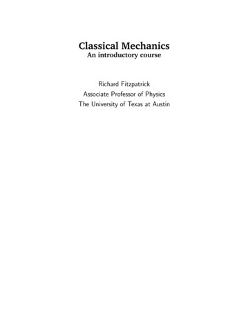
CHAPTER 1. ANALYTICAL MECHANICS14Theorem 1.4.1. There are only 2 types of central potentials in which all solutions(associated trajectories) are closed. These potentials take the form:αU (r) ,rU (r) αr2 ,(1.65a)(1.65b)where α 0.There is a caveat when working with Eq. (1.64), and that it we must require thatH Ueff (r),(1.66)within the bounds of integration, so that the equation is well defined. To ground this intuitiona little, we consider the specific potential where U (r) α/r, which grants thatUeff (r) α 2 .2µr2r(1.67)Potentials of such form look like the illustration in Fig. 1.2.Figure 1.2: Effective potential curve with U (r) α/r.We can see that there are several regimes in which the value of E can place the system in, whichhas been discussed equivalently from the result of Kepler’s first law in Sec. 1.4.2 (pertaining to theeccentricity of the orbits). If we consider the energy regime where E Eellipse , we will retrieveEq. (1.58) from Eq. (1.64) after evaluating the integrals appropriately. Using the parameters inFig. 1.2, the shape of the trajectory can also be written asA,1 e cos φxmax xminxmax xminA , e .2xmax xminr(φ) where(1.68)(1.69)It is also not too hard to derive for bounded orbits (E 0), the boundary points xmax and xmin

151.4. CENTRAL POTENTIALSasrµαµ2 α22µExmax 2 , 2 4 r22µα2µEµ αxmin 2 , 2 4 (1.70a)(1.70b)by setting the denominator in the integrand of Eq. (1.64) to zero. From this, we see that we getcircular orbits when:E µα2,2 2(1.71)that results in e 0 and r A. More on the geometry of the ellipse, the center of the ellipse islocated a distance ed A,(1.72)1 e2from the focus along the line joining the 2 foci. In Cartesian coordinates, the ellipse can bewritten asx2(y d)2 1,2ab2(1.73)where a is the semi-major axis, b the semi-minor axis and the origin is set at the lower focuswith y aligned to the line joining the 2 foci. Explicitly, the semi-major and semi-minor axes canbe calculated to beA,1 e2Ab .1 e2a (1.74a)(1.74b)For these bounded orbits, one could also ask how long it would take to complete one revolution.This can be easily found from the angular momentum

Chapter 1 Analytical Mechanics Classical mechanics is a very old subject and is the basis for many other elds of physics one would bump into. Most famously, classical mechanics is built upon Newton's 3 laws, which involve