WIXLIB

IntroductionForward-Backward ProcedureViterbi AlgorithmBaum-Welch ReestimationExtensionsA Tutorial on Hidden Markov Modelsby Lawrence R. Rabinerin Readings in speech recognition (1990)Marcin MarszalekVisual Geometry Group16 February 2009Figure: Andrey MarkovMarcin MarszalekA Tutorial on Hidden Markov Models

IntroductionForward-Backward ProcedureViterbi AlgorithmBaum-Welch ReestimationExtensionsSignals and signal modelsReal-world processes produce signals, i.e., observable outputsdiscrete (from a codebook) vs continousstationary (with const. statistical properties) vs nonstationarypure vs corrupted (by noise)Signal models provide basis forsignal analysis, e.g., simulationsignal processing, e.g., noise removalsignal recognition, e.g., identificationSignal models can bedeterministic – exploit some known properties of a signalstatistical – characterize statistical properties of a signalStatistical signal modelsGaussian processesPoisson processesMarcin MarszalekMarkov processesHidden Markov processesA Tutorial on Hidden Markov Models

IntroductionForward-Backward ProcedureViterbi AlgorithmBaum-Welch ReestimationExtensionsSignals and signal modelsReal-world processes produce signals, i.e., observable outputsdiscrete (from a codebook) vs continousstationary (with const. statistical properties) vs nonstationarypure vs corrupted (by noise)Signal models provide basis forAssumptione.g., simulationSignal signalcan beanalysis,well characterizedas a parametric randomsignal processing, e.g., noise removalprocess, and the parameters of the stochastic process can besignal recognition, e.g., identificationdetermined in a precise, well-defined mannerSignal models can bedeterministic – exploit some known properties of a signalstatistical – characterize statistical properties of a signalStatistical signal modelsGaussian processesPoisson processesMarcin MarszalekMarkov processesHidden Markov processesA Tutorial on Hidden Markov Models

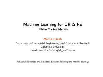
IntroductionForward-Backward ProcedureViterbi AlgorithmBaum-Welch ReestimationDiscrete (observable) Markov modelFigure: A Markov chain with 5 states and selected transitionsN states: S1 , S2 , ., SNIn each time instant t 1, 2, ., T a system changes(makes a transition) to state qtMarcin MarszalekA Tutorial on Hidden Markov ModelsExtensions

IntroductionForward-Backward ProcedureViterbi AlgorithmBaum-Welch ReestimationExtensionsDiscrete (observable) Markov modelFor a special case of a first order Markov chainP(qt Sj qt 1 Si , tt 2 Sk , .) P(qt Sj qt 1 Si )Furthermore we only assume processes where right-hand sideis time independent – const. state transition probabilitiesaij P(qt Sj qt 1 Sj )whereaij 0NX1 i, j Naij 1j 1Marcin MarszalekA Tutorial on Hidden Markov Models

IntroductionForward-Backward ProcedureViterbi AlgorithmBaum-Welch ReestimationDiscrete hidden Markov model (DHMM)Figure: Discrete HMM with 3 states and 4 possible outputsAn observation is a probabilistic function of a state, i.e.,HMM is a doubly embedded stochastic processA DHMM is characterized byN states Sj and M distinct observations vk (alphabet size)State transition probability distribution AObservation symbol probability distribution BInitial state distribution πMarcin MarszalekA Tutorial on Hidden Markov ModelsExtensions

IntroductionForward-Backward ProcedureViterbi AlgorithmBaum-Welch ReestimationDiscrete hidden Markov model (DHMM)We define the DHMM as λ (A, B, π)A {aij }B {bik }aij P(qt 1 Sj qt Si )bik P(Ot vk qt Si )π {πi }πi P(q1 Si )1 i, j N1 i N1 k M1 i NThis allows to generate an observation seq. O O1 O2 .OT1234Set t 1, choose an initial state q1 Si according to theinitial state distribution πChoose Ot vk according to the symbol probabilitydistribution in state Si , i.e., bikTransit to a new state qt 1 Sj accordingto the state transition probability distibutionfor state Si , i.e., aijSet t t 1,if t T then return to step 2Marcin MarszalekA Tutorial on Hidden Markov ModelsExtensions

IntroductionForward-Backward ProcedureViterbi AlgorithmBaum-Welch ReestimationExtensionsThree basic problems for HMMsEvaluation Given the observation sequence O O1 O2 .OT anda model λ (A, B, π), how do we efficientlycompute P(O λ), i.e., the probability of theobservation sequence given the modelRecognition Given the observation sequence O O1 O2 .OT anda model λ (A, B, π), how do we choose acorresponding state sequence Q q1 q2 .qT which isoptimal in some sense, i.e., best explains theobservationsTraining Given the observation sequence O O1 O2 .OT , howdo we adjust the model parameters λ (A, B, π) tomaximize P(O λ)Marcin MarszalekA Tutorial on Hidden Markov Models

IntroductionForward-Backward ProcedureViterbi AlgorithmBaum-Welch ReestimationBrute force solution to the evaluation problemWe need P(O λ), i.e., the probability of the observationsequence O O1 O2 .OT given the model λSo we can enumerate every possible state sequenceQ q1 q2 .qTFor a sample sequence QP(O Q, λ) TYt 1P(Ot qt , λ) TYbqt Ott 1The probability of such a state sequence Q isP(Q λ) P(q1 )TYt 2Marcin MarszalekP(qt qt 1 ) πq1TYaqt 1 qtt 2A Tutorial on Hidden Markov ModelsExtensions

IntroductionForward-Backward ProcedureViterbi AlgorithmBaum-Welch ReestimationBrute force solution to the evaluation problemTherefore the joint probabilityP(O, Q λ) P(Q λ)P(O Q, λ) πq1TYaqt 1 qtt 2TYt 1By considering all possible state sequencesP(O λ) Xπq1 bq1 O1QTYaqt 1 qt bqt Ott 2Problem: order of 2TN T calculationsN T possible state sequencesabout 2T calculations for each sequenceMarcin MarszalekA Tutorial on Hidden Markov Modelsbqt OtExtensions

IntroductionForward-Backward ProcedureViterbi AlgorithmBaum-Welch ReestimationForward procedureWe define a forward variable αj (t) as the probability of thepartial observation seq. until time t, with state Sj at time tαj (t) P(O1 O2 .Ot , qt Sj λ)This can be computed inductively1 j Nαj (1) πj bjO1αj (t 1) NX αi (t)aij bjOt 11 t T 1i 1Then with N 2 T operations:P(O λ) NXP(O, qT Si λ) i 1Marcin MarszalekNXαi (T )i 1A Tutorial on Hidden Markov ModelsExtensions

IntroductionForward-Backward ProcedureViterbi AlgorithmBaum-Welch ReestimationForward procedureFigure: Operations forcomputing the forwardvariable αj (t 1)Figure: Computing αj (t)in terms of a latticeMarcin MarszalekA Tutorial on Hidden Markov ModelsExtensions

IntroductionForward-Backward ProcedureViterbi AlgorithmBaum-Welch ReestimationBackward procedureFigure: Operations forcomputing the backwardvariable βi (t)We define a backwardvariable βi (t) as theprobability of the partialobservation seq. after time t, given state Si at time tβi (t) P(Ot 1 Ot 2.OT qt Si , λ)This can be computed inductively as well1 i Nβi (T ) 1βi (t 1) NXaij bjOt βj (t)2 t Tj 1Marcin MarszalekA Tutorial on Hidden Markov ModelsExtensions

IntroductionForward-Backward ProcedureViterbi AlgorithmBaum-Welch ReestimationExtensionsUncovering the hidden state sequenceUnlike for evaluation, there is no single “optimal” sequenceChoose states which are individually most likely(maximizes the number of correct states)Find the single best state sequence(guarantees that the uncovered sequence is valid)The first choice means finding argmaxi γi (t) for each t, whereγi (t) P(qt Si O, λ)In terms of forward and backward variablesP(O1 .Ot , qt Si λ)P(Ot 1 .OT qt Si , λ)P(O λ)αi (t)βi (t)γi (t) PNj 1 αj (t)βj (t)γi (t) Marcin MarszalekA Tutorial on Hidden Markov Models

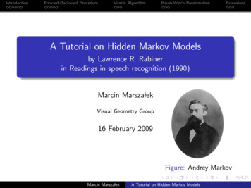
IntroductionForward-Backward ProcedureViterbi AlgorithmBaum-Welch ReestimationExtensionsViterbi algorithmFinding the best single sequence means computingargmaxQ P(Q O, λ), equivalent to argmaxQ P(Q, O λ)The Viterbi algorithm (dynamic programming) defines δj (t),i.e., the highest probability of a single path of length t whichaccounts for the observations and ends in state Sjδj (t) maxq1 ,q2 ,.,qt 1P(q1 q2 .qt j, O1 O2 .Ot λ)By induction1 j Nδj (1) πj bjO1 δj (t 1) max δi (t)aij bjOt 1i1 t T 1With backtracking (keeping the maximizing argument for eacht and j) we find the optimal solutionMarcin MarszalekA Tutorial on Hidden Markov Models

IntroductionForward-Backward ProcedureViterbi AlgorithmBaum-Welch ReestimationBacktrackingFigure: Illustration of the backtracking procedure c G.W. PulfordMarcin MarszalekA Tutorial on Hidden Markov ModelsExtensions

IntroductionForward-Backward ProcedureViterbi AlgorithmBaum-Welch ReestimationExtensionsEstimation of HMM parametersThere is no known way to analytically solve for the modelwhich maximizes the probability of the observation sequenceWe can choose λ (A, B, π) which locally maximizes P(O λ)gradient techniquesBaum-Welch reestimation (equivalent to EM)We need to define ξij (t), i.e., the probability of being in stateSi at time t and in state Sj at time t 1ξij (t) P(qt Si , qt 1 Sj O, λ)αi (t)aij bjOt 1 βj (t 1)ξij (t) P(O λ)αi (t)aij bjOt 1 βj (t 1) PN PNi 1j 1 αi (t)aij bjOt 1 βj (t 1)Marcin MarszalekA Tutorial on Hidden Markov Models

IntroductionForward-Backward ProcedureViterbi AlgorithmBaum-Welch ReestimationEstimation of HMM parametersFigure: Operations forcomputing the ξij (t)Recall that γi (t) is a probability of state Si at time t, henceγi (t) NXξij (t)j 1Now if we sum over the time index tPT 1γi (t) expected number of times that Si is visited expected number of transitions from state SiPT 1ξ(t) expected number of transitions from Si to Sjijt 1t 1Marcin MarszalekA Tutorial on Hidden Markov ModelsExtensions

IntroductionForward-Backward ProcedureViterbi AlgorithmBaum-Welch ReestimationExtensionsBaum-Welch ReestimationReestimation formulasPT 1π̄i γi (1)a ij t 1 ξij (t)PT 1t 1 γi (t)PO v γj (t)b jk PTt kt 1 γj (t)Baum et al. proved that if current model is λ (A, B, π) andwe use the above to compute λ̄ (Ā, B̄, π̄) then eitherλ̄ λ – we are in a critical point of the likelihood functionP(O λ̄) P(O λ) – model λ̄ is more likelyIf we iteratively reestimate the parameters we obtain amaximum likelihood estimate of the HMMUnfortunately this finds a local maximum and the surface canbe very complexMarcin MarszalekA Tutorial on Hidden Markov Models

IntroductionForward-Backward ProcedureViterbi AlgorithmBaum-Welch ReestimationNon-ergodic HMMsUntil now we have only consideredergodic (fully connected) HMMsevery state can be reached fromany state in a finite number ofstepsFigure: Ergodic HMMLeft-right (Bakis) model good for speech recognitionas time increases the state index increases or stays the samecan be extended to parallel left-right modelsFigure: Left-right HMMFigure: Parallel HMMMarcin MarszalekA Tutorial on Hidden Markov ModelsExtensions

IntroductionForward-Backward ProcedureViterbi AlgorithmBaum-Welch ReestimationGaussian HMM (GMMM)HMMs can be used with continous observation densitiesWe can model such densities with Gaussian mixturesbjO MXcjm N (O, µjm , Ujm )m 1Then the reestimation formulas are still simpleMarcin MarszalekA Tutorial on Hidden Markov ModelsExtensions

IntroductionForward-Backward ProcedureViterbi AlgorithmBaum-Welch ReestimationMore funAutoregressive HMMsState Duration Density HMMsDiscriminatively trained HMMsmaximum mutual informationinstead of maximum likelihoodHMMs in a similarity measureConditional Random Fields canloosely be understood as ageneralization of an HMMsFigure: Random Oxfordfields c R. Tourtelotconstant transition probabilities replaced with arbitraryfunctions that vary across the positions in the sequence ofhidden statesMarcin MarszalekA Tutorial on Hidden Markov ModelsExtensions

A Tutorial on Hidden Markov Models by Lawrence R. Rabiner in Readings in speech recognition (1990) Marcin Marsza lek Visual Geometry Group . { we are in a critical point of the likelihood function P(Oj ) P(Oj ) { model is more likely. If we iteratively reestimate the parameters we obtain a