Transcription
SADDLE-POINT DYNAMICS: CONDITIONS FOR ASYMPTOTICSTABILITY OF SADDLE POINTS ASHISH CHERUKURI† , BAHMAN GHARESIFARD‡ , AND JORGE CORTÉS†Abstract. This paper considers continuously differentiable functions of two vector variablesthat have (possibly a continuum of) min-max saddle points. We study the asymptotic convergenceproperties of the associated saddle-point dynamics (gradient-descent in the first variable and gradientascent in the second one). We identify a suite of complementary conditions under which the set ofsaddle points is asymptotically stable under the saddle-point dynamics. Our first set of results isbased on the convexity-concavity of the function defining the saddle-point dynamics to establish theconvergence guarantees. For functions that do not enjoy this feature, our second set of results relieson properties of the linearization of the dynamics, the function along the proximal normals to thesaddle set, and the linearity of the function in one variable. We also provide global versions of theasymptotic convergence results. Various examples illustrate our discussion.Key words. saddle-point dynamics, asymptotic convergence, convex-concave functions, proximal calculus, center manifold theory, nonsmooth dynamicsAMS subject classifications. 34A34, 34D05, 34D23, 34D35, 37L101. Introduction. It is well known that the trajectories of the gradient dynamicsof a continuously differentiable function with bounded sublevel sets converge asymptotically to its set of critical points, see e.g. [20]. This fact, however, is not true ingeneral for the saddle-point dynamics (gradient descent in one variable and gradient ascent in the other) of a continuously differentiable function of two variables, seee.g. [2, 13]. In this paper, our aim is to investigate conditions under which the abovestatement is true for the case where the critical points are min-max saddle pointsand they possibly form a continuum. Our motivation comes from the applications ofthe saddle-point dynamics (also known as primal-dual dynamics) to find solutions ofequality constrained optimization problems and Nash equilibria of zero-sum games.Literature review. In constrained optimization problems, the pioneering works [2,25] popularized the use of the primal-dual dynamics to arrive at the saddle points ofthe Lagrangian. For inequality constrained problems, this dynamics is modified witha projection operator on the dual variables to preserve their nonnegativity, whichresults in a discontinuous vector field. Recent works have further explored the convergence analysis of such dynamics, both in continuous [17, 9] and in discrete [27]time. The work [16] proposes instead a continuous dynamics whose design builds onfirst- and second-order information of the Lagrangian. In the context of distributedcontrol and multi-agent systems, an important motivation to study saddle-point dynamics comes from network optimization problems where the objective function is anaggregate of each agents’ local objective function and the constraints are given by aset of conditions that are locally computable at the agent level. Because of this structure, the saddle-point dynamics of the Lagrangian for such problems is inherentlyamenable to distributed implementation. This observation explains the emerging† Department of Mechanical and Aerospace Engineering, University of California, San Diego, 9500Gilman Dr., La Jolla, CA 92093-0411, United States, {acheruku,cortes}@ucsd.edu‡ Department of Mathematics and Statistics, Queen’s University, 403 Jeffery Hall, UniversityAve., Kingston, ON, Canada K7L3N6, bahman@mast.queensu.ca A preliminary version of this paper appeared at the 2015 American Control Conference as [8].1
body of work that, from this perspective, looks at problems in distributed convex optimization [33, 18, 14], distributed linear programming [30], and applications to powernetworks [26, 34, 35] and bargaining problems [31]. The work [23] shows an interestingapplication of the saddle-point dynamics to find a common Lyapunov function for alinear differential inclusion. In game theory, it is natural to study the convergenceproperties of saddle-point dynamics to find the Nash equilibria of two-person zero-sumgames [3, 29]. A majority of these works assume the function whose saddle pointsare sought to be convex-concave in its arguments. Our focus here instead is on theasymptotic stability of the min-max saddle points under the saddle-point dynamicsfor a wider class of functions, and without any nonnegativity-preserving projection onindividual variables. We explicitly allow for the possibility of a continuum of saddlepoints, instead of isolated ones, and wherever feasible, on establishing convergence ofthe trajectories to a point in the set. The issue of asymptotic convergence, even inthe case of standard gradient systems, is a delicate one when equilibria are a continuum [1]. In such scenarios, convergence to a point might not be guaranteed, see e.g.,the counter example in [28]. Our work here is complementary to [21], which focuseson the characterization of the asymptotic behavior of the saddle-point dynamics whentrajectories do not converge to saddle points and instead show oscillatory behaviour.Statement of contributions. Our starting point is the definition of the saddlepoint dynamics for continuously differentiable functions of two (vector) variables,which we term saddle functions. The saddle-point dynamics consists of gradient descent of the saddle function in the first variable and gradient ascent in the secondvariable. Our objective is to characterize the asymptotic convergence properties ofthe saddle-point dynamics to the set of min-max saddle points of the saddle function.Assuming this set is nonempty, our contributions can be understood as a catalog ofcomplementary conditions on the saddle function that guarantee that the trajectoriesof the saddle-point dynamics are proved to converge to the set of saddle points, andpossibly to a point in the set. We broadly divide our results in two categories, one inwhich the saddle function has convexity-concavity properties and the other in which itdoes not. For the first category, our starting result considers saddle functions that arelocally convex-concave on the set of saddle points. We show that asymptotic stabilityof the set of saddle points is guaranteed if either the convexity or concavity properties are strict, and convergence is pointwise. Furthermore, motivated by equalityconstrained optimization problems, our second result shows that the same conclusionson convergence hold for functions that depend linearly on one of its arguments if thestrictness requirement is dropped. For the third and last result in this category, werelax the convexity-concavity requirement and establish asymptotic convergence forstrongly jointly quasiconvex-quasiconcave saddle functions. Moving on to the secondcategory of scenarios, where functions lack convexity-concavity properties, our firstcondition is based on linearization. We consider piecewise twice continuously differentiable saddle-point dynamics and provide conditions on the eigenvalues of the limitpoints of Jacobian matrices of the saddle function at the saddle points that ensurelocal asymptotic stability of a manifold of saddle points. Our convergence analysisis based on a general result of independent interest on the stability of a manifoldof equilibria for piecewise smooth vector fields that we state and prove using ideasfrom center manifold theory. The next two results are motivated by the observationthat saddle functions exist in the second category that do not satisfy the linearizationhypotheses and yet have convergent dynamics. In one result, we justify convergenceby studying the variation of the function and its Hessian along the proximal normal2
directions to the set of saddle points. Specifically, we assume polynomial bounds forthese variations and derive an appropriate relationship between these bounds thatensures asymptotic convergence. In the other result, we assume the saddle functionto be linear in one variable and indefinite in another, where the indefinite part satisfiessome appropriate regularity conditions. When discussing each of the above scenarios,we extend the conditions to obtain global convergence wherever feasible. Our analysis is based on tools and notions from saddle points, stability analysis of nonlinearsystems, proximal normals, and center manifold theory. Various illustrative examplesthroughout the paper justify the complementary character of the hypotheses in ourresults.Organization. Section 2 introduces notation and basic preliminaries. Section 3presents the saddle-point dynamics and the problem statement. Section 4 deals withsaddle functions with convexity-concavity properties. For the case when this propertydoes not hold, Section 5 relies on linearization techniques, proximal normals, and thelinearity structure of the saddle function to establish convergence guarantees. Finally,Section 6 summarizes our conclusions and ideas for future work.2. Preliminaries. This section introduces basic notation and presents preliminaries on proximal calculus and saddle points.2.1. Notation. We let R, R 0 , R 0 , R 0 and Z 1 be the set of real, nonnegativereal, nonpositive real, positive real, and positive integer numbers, respectively. Giventwo sets A1 , A2 Rn , we let A1 A2 {x y x A1 , y A2 }. We denote byk · k the 2-norm on Rn and also the induced 2-norm on Rn n . Let Bδ (x) representthe open ball centered at x Rn of radius δ 0. Given x Rn , xi denotes thei-th component of x. For vectors u Rn and w Rm , the vector (u; w) Rn mdenotes their concatenation. For A Rn n , we use A 0, A 0, A 0, andA 0 to denote the fact that A is positive semidefinite, negative semidefinite, positivedefinite, and negative definite, respectively. The eigenvalues of A are λi (A) for i {1, . . . , n}. If A is symmetric, λmax (A) and λmin (A) represent the maximum andminimum eigenvalues, respectively. The range and null spaces of A are denoted byrange(A), null(A), respectively. We use the notation C k for a function being k Z 1times continuously differentiable. A set S Rn is path connected if for any two pointsa, b S there exists a continuous map γ : [0, 1] S such that γ(0) a and γ(1) b.A set Sc S Rn is an isolated path connected component of S if it is path connectedand there exists an open neighborhood U of Sc in Rn such that U S Sc . For areal-valued function F : Rn Rm R, we denote the partial derivative of F withrespect to the first argument by x F and with respect to the second argument by2 2F, xx F xF2 , z F . The higher-order derivatives follow the convention xz F x znmnand so on. The restriction of f : R R to a subset S R is denoted by f S .The Jacobian of a C 1 map f : Rn Rm at x Rn is denoted by Df (x) Rm n .For a real-valued function V : Rn R and α 0, we denote the sublevel set of Vby V 1 ( α) {x Rn V (x) α}. Finally, a vector field f : Rn Rn is saidto be piecewise C 2 if it is continuous and there exists (1) a finite collection of disjointopen sets D1 , . . . , Dm Rn , referred to as patches, whose closure covers Rn , that is,2en mRn mi 1 cl(Di ) and (2) a finite collection of C functions {fi : Di R }i 1 where,eefor each i {1, . . . , m}, Di is open with cl(Di ) Di , such that f cl(Di ) and fi takethe same values over cl(Di ).3
2.2. Proximal calculus. We present here a few notions on proximal calculusfollowing [11]. Given a closed set E Rn and a point x Rn \E, the distance from xto E is,(2.1)dE (x) min kx yk.y EWe let projE (x) denote the set of points in E that are closest to x, i.e., projE (x) {y E kx yk dE (x)} E. For y projE (x), the vector x y is a proximal normaldirection to E at y and any nonnegative multiple ζ t(x y), t 0 is called a proximalnormal (P -normal) to E at y. The distance function dE might not be differentiablein general (unless E is convex), but is globally Lipschitz and regular [11, p. 23]. Fora locally Lipschitz function f : Rn R, the generalized gradient f : Rn Rn is f (x) co{ lim f (xi ) xi x, xi / S Ωf },i where co denotes convex hull, S Rn is any set of measure zero, and Ωf is the set(of measure zero) of points where f is not differentiable. In the case of the square ofthe distance function, one can compute [11, p. 99] the generalized gradient as,(2.2) d2E (x) co{2(x y) y projE (x)}.2.3. Saddle points. Here, we provide basic definitions pertaining to the notionof saddle points. A point (x , z ) Rn Rm is a local min-max saddle point of a continuously differentiable function F : Rn Rm R if there exist open neighborhoodsUx Rn of x and Uz Rm of z such that(2.3)F (x , z) F (x , z ) F (x, z ),for all z Uz and x Ux . The point (x , z ) is a global min-max saddle point of Fif Ux Rn and Uz Rm . Min-max saddle points are a particular case of the moregeneral notion of saddle points. We focus here on min-max saddle points motivated byproblems in constrained optimization and zero-sum games, whose solutions correspondto min-max saddle points. With a slight abuse of terminology, throughout the paperwe refer to the local min-max saddle points simply as saddle points. We denote bySaddle(F ) the set of saddle points of F . From (2.3), for (x , z ) Saddle(F ), thepoint x Rn (resp. z Rm ) is a local minimizer (resp. local maximizer) of themap x 7 F (x, z ) (resp. z 7 F (x , z)). Each saddle point is a critical point of F , i.e., x F (x , z ) 0 and z F (x , z ) 0. Additionally, if F is C 2 , then xx F (x , z ) 0and zz F (x , z ) 0. Also, if xx F (x , z ) 0 and zz F (x , z ) 0, then theinequalities in (2.3) are strict.A function F : Rn Rm R is locally convex-concave at a point (x̃, z̃) Rn Rmif there exists an open neighborhood U of (x̃, z̃) such that for all (x̄, z̄) U, thefunctions x 7 F (x, z̄) and z 7 F (x̄, z) are convex over U (Rn {z̄}) and concaveover U ({x̄} Rm ), respectively. If in addition, either x 7 F (x, z̃) is strictlyconvex in an open neighborhood of x̃, or z 7 F (x̃, z) is strictly concave in an openneighborhood of z̃, then F is locally strictly convex-concave at (x̃, z̃). F is locally (resp.locally strictly) convex-concave on a set S Rn Rm if it is so at each point in S. Fis globally convex-concave if in the local definition U Rn Rm . Finally, F is globallystrictly convex-concave if it is globally convex-concave and for any (x̄, z̄) Rn Rm ,either x 7 F (x, z̄) is strictly convex or z 7 F (x̄, z) is strictly concave. Note that this4
notion is different than saying that F is both strictly convex and strictly concave.Next, we define strongly quasiconvex function following [22]. A function f : Rn R is strongly quasiconvex with parameter s 0 over a convex set D Rn if for allx, y D and all λ [0, 1] we have,max{f (x), f (y)} f (λx (1 λ)y) sλ(1 λ)kx yk2 .A function f is strongly quasiconcave with parameter s 0 over the set D if f isstrongly quasiconvex with parameter s over D. A function F : Rn Rm R is locallyjointly strongly quasiconvex-quasiconcave at a point (x̃, z̃) Rn Rm if there exists 0 and an open neighborhood U of (x̃, z̃) such that for all (x̄, z̄) U, the functionx 7 F (x, z̄) is strongly quasiconvex with parameter s over U (Rn {z̄}) and thefunction z 7 F (x̄, z) is strongly quasiconvex with parameter s over U ({x̄} Rm ).F is locally jointly strongly quasiconvex-quasiconcave on a set S Rn Rm if it isso at each point in S. F is globally jointly strongly quasiconvex-quasiconcave if in thelocal definition U Rn Rm .3. Problem statement. Here we formulate the problem of interest in the paper.Given a continuously differentiable function F : Rn Rm R, which we refer to assaddle function, we consider its saddle-point dynamics, i.e., gradient-descent in oneargument and gradient-ascent in the other,(3.1a)ẋ x F (x, z),(3.1b)ż z F (x, z).When convenient, we use the shorthand notation Xsp : Rn Rm Rn Rm to referto this dynamics. Our aim is to provide conditions on F under which the trajectoriesof its saddle-point dynamics (3.1) locally asymptotically converge to its set of saddlepoints, and possibly to a point in the set. We are also interested in identifyingconditions to establish global asymptotic convergence. Throughout our study, weassume that the set Saddle(F ) is nonempty. This assumption is valid under mildconditions in the application areas that motivate our study: for the Lagrangian of theconstrained optimization problem [6] and the value function for zero-sum games [3].Our forthcoming discussion is divided in two threads, one for the case of convexconcave functions, cf. Section 4, and one for the case of general functions, cf. Section 5.In each case, we provide illustrative examples to show the applicability of the results.4. Convergence analysis for convex-concave saddle functions. This section presents conditions for the asymptotic stability of saddle points under the saddlepoint dynamics (3.1) that rely on the convexity-concavity properties of the saddlefunction.4.1. Stability under strict convexity-concavity. Our first result providesconditions that guarantee the local asymptotic stability of the set of saddle points.Proposition 4.1. (Local asymptotic stability of the set of saddle points viaconvexity-concavity): For F : Rn Rm R continuously differentiable and locally strictly convex-concave on Saddle(F ), each isolated path connected componentof Saddle(F ) is locally asymptotically stable under the saddle-point dynamics Xspand, moreover, the convergence of each trajectory is to a point.Proof. Let S be an isolated path connected component of Saddle(F ) and take(x , z ) S. Without loss of generality, we consider the case when x 7 F (x, z ) is5
locally strictly convex (the proof for the case when z 7 F (x , z) is locally strictlyconcave is analogous). Consider the function V : Rn Rm R 0 ,(4.1)V (x, z) 1 kx x k2 kz z k2 ,2which we note is radially unbounded (and hence has bounded sublevel sets). Werefer to V as a LaSalle function because locally, as we show next, its Lie derivativeis negative, but not strictly negative. Let U be the neighborhood of (x , z ) wherelocal convexity-concavity holds. The Lie derivative of V along the dynamics (3.1) at(x, z) U can be written as,(4.2)LXsp V (x, z) (x x ) x F (x, z) (z z ) z F (x, z), F (x , z) F (x, z) F (x, z) F (x, z ), F (x , z) F (x , z ) F (x , z ) F (x, z ) 0,where the first inequality follows from the first-order condition for convexity andconcavity, and the last inequality follows from the definition of saddle point. Asa consequence, for α 0 small enough such that V 1 ( α) U, we concludethat V 1 ( α) is positively invariant under Xsp . The application of the LaSalleInvariance Principle [24, Theorem 4.4] yields that any trajectory starting from apoint in V 1 ( α) converges to the largest invariant set M contained in {(x, z) V 1 ( α) LXsp V (x, z) 0}. Let (x, z) M . From (4.2), LXsp V (x, z) 0 implies that F (x , z) F (x , z ) F (x, z ). In turn, the local strict convexity ofx 7 F (x, z ) implies that x x . Since M is positively invariant, the trajectoryt 7 (x(t), z(t)) of Xsp starting at (x, z) is contained in M . This implies that alongthe trajectory, for all t 0, (a) x(t) x i.e., ẋ(t) x F (x(t), z(t)) 0, and (b)F (x , z(t)) F (x , z ). The later implies0 LXsp F (x , z(t)) Xsp (x , z(t)) · (0, z F (x , z(t))) k z F (x(t), z(t))k2 ,for all t 0. Thus, we get x F (x, z) 0 and z F (x, z) 0. Further, since(x, z) U, local convexity-concavity holds over U, and S is an isolated component,we obtain (x, z) S, which shows M S. Since (x , z ) is arbitrary, the asymptoticconvergence property holds in a neighborhood of S. The pointwise convergence followsfrom the application of Lemma A.3.The result above shows that each saddle point is stable and that each path connected component of Saddle(F ) is asymptotically stable. Note that each saddle pointmight not be asymptotically stable. However, if a component consists of a singlepoint, then that point is asymptotically stable. Interestingly, a close look at the proofof Proposition 4.1 reveals that, if the assumptions hold globally, then the asymptoticstability of the set of saddle points is also global, as stated next.Corollary 4.2. (Global asymptotic stability of the set of saddle points viaconvexity-concavity): For F : Rn Rm R continuously differentiable and globallystrictly convex-concave, Saddle(F ) is globally asymptotically stable under the saddlepoint dynamics Xsp and the convergence of trajectories is to a point.Remark 4.3. (Relationship with results on primal-dual dynamics: I): Corollary 4.2 is an extension to more general functions and less stringent assumptions ofthe results stated for Lagrangian functions of constrained convex (or concave) optimization problems in [33, 2, 17] and cost functions of differential games in [29].6
In [2, 17], for a concave optimization, the matrix xx F is assumed to be negativedefinite at every saddle point and in [33] the set Saddle(F ) is assumed to be a singleton. The work [29] assumes a sufficient condition on the cost functions to guaranteeconvergence that in the current setup is equivalent to having xx F and zz F positiveand negative definite, respectively. 4.2. Stability under convexity-linearity or linearity-concavity. Here westudy the asymptotic convergence properties of the saddle-point dynamics when theconvexity-concavity of the saddle function is not strict but, instead, the function depends linearly on its second argument. The analysis follows analogously for saddlefunctions that are linear in the first argument and concave in the other. The consideration of this class of functions is motivated by equality constrained optimizationproblems.Proposition 4.4. (Local asymptotic stability of the set of saddle points viaconvexity-linearity): For a continuously differentiable function F : Rn Rm R, if(i) F is locally convex-concave on Saddle(F ) and linear in z,(ii) for each (x , z ) Saddle(F ), there exists a neighborhood Ux Rn of x where, if F (x, z ) F (x , z ) with x Ux , then (x, z ) Saddle(F ),then each isolated path connected component of Saddle(F ) is locally asymptoticallystable under the saddle-point dynamics Xsp and, moreover, the convergence of trajectories is to a point.Proof. Given an isolated path connected component S of Saddle(F ), Lemma A.1implies that F S is constant. Our proof proceeds along similar lines as those of Proposition 4.1. With the same notation, given (x , z ) S, the arguments follow verbatim until the identification of the largest invariant set M contained in {(x, z) V 1 ( α) LXsp V (x, z) 0}. Let (x, z) M . From (4.2), LXsp V (x, z) 0 impliesF (x , z) F (x , z ) F (x, z ). By assumption (ii), this means (x, z ) S, and byassumption (i), the linearity property gives z F (x, z) z F (x, z ) 0. Therefore z F M 0. For (x, z) M , the trajectory t 7 (x(t), z(t)) of Xsp starting at (x, z) iscontained in M . Consequently, z(t) z for all t [0, ) and ẋ(t) x F (x(t), z)corresponds to the gradient dynamics of the (locally) convex function y 7 F (y, z).Therefore, x(t) converges to a minimizer x0 of this function, i.e., x F (x0 , z) 0.Since z F M 0, the continuity of z F implies that z F (x0 , z) 0, and hence(x0 , z) S. By continuity of F , it follows that F (x(t), z) F (x0 , z) F (x , z ),where for the equality we use the fact that F S is constant. On the other hand, notethat 0 LXsp V (x(t), z) (x(t) x ) x F (x(t), z) F (x , z) F (x(t), z) impliesF (x(t), z) F (x , z) F (x , z ),for all t [0, ). Therefore, the monotonically nonincreasing sequence {F (x(t), z)}converges to F (x , z ), which is also an upper bound on the whole sequence. Thiscan only be possible if F (x(t), z) F (x , z ) for all t [0, ). This further implies x F (x(t), z) 0 for all t [0, ), and hence, (x, z) S. Consequently, M S. Since (x , z ) has been chosen arbitrarily, the convergence property holds in aneighborhood of S. The pointwise convergence follows now from the application ofLemma A.3.The assumption (ii) in the above result is a generalization of the local strictconvexity condition for the function F (·, z ). That is, (ii) allows other points in theneighborhood of x to have the same value of the function F (·, z ) as that at x , as long7
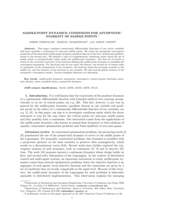
as they are saddle points (whereas, under local strict convexity, x is the local uniqueminimizer of F (·, z )). The next result extends the conclusions of Proposition 4.4globally when the assumptions hold globally.Corollary 4.5. (Global asymptotic stability of the set of saddle points viaconvexity-linearity): For a C 1 function F : Rn Rm R, if(i) F is globally convex-concave and linear in z,(ii) for each (x , z ) Saddle(F ), if F (x, z ) F (x , z ), then (x, z ) Saddle(F ),then Saddle(F ) is globally asymptotically stable under the saddle-point dynamics Xspand, moreover, convergence of trajectories is to a point.Example 4.6. (Saddle-point dynamics for convex optimization): Consider thefollowing convex optimization problem on R3 ,(4.3a)(4.3b)minimize(x1 x2 x3 )2 ,subject to x1 x2 .The set of solutions of this optimization is {x R3 2x1 x3 0, x2 x1 }, withLagrangian(4.4)L(x, z) (x1 x2 x3 )2 z(x1 x2 ),where z R is the Lagrange multiplier. The set of saddle points of L (whichcorrespond to the set of primal-dual solutions to (4.3)) are Saddle(L) {(x, z) R3 R 2x1 x3 0, x1 x2 , and z 0}. However, L is not strictly convexconcave and hence, it does not satisfy the hypotheses of Corollary 4.2. While L isglobally convex-concave and linear in z, it does not satisfy assumption (ii) of Corollary 4.5. Therefore, to identify a dynamics that renders Saddle(L) asymptoticallystable, we form the augmented Lagrangian(4.5)L̃(x, z) L(x, z) (x1 x2 )2 ,that has the same set of saddle points as L. Note that L̃ is not strictly convex-concavebut it is globally convex-concave (this can be seen by computing its Hessian) and islinear in z. Moreover, given any (x , z ) Saddle(L), we have L̃(x , z ) 0, and ifL̃(x, z ) L̃(x , z ) 0, then (x, z ) Saddle(L). By Corollary 4.5, the trajectoriesof the saddle-point dynamics of L̃ converge to a point in S and hence, solve theoptimization problem (4.3). Figure 4.1 illustrates this fact. Note that the point ofconvergence depends on the initial condition. Remark 4.7. (Relationship with results on primal-dual dynamics: II): Thework [17, Section 4] considers concave optimization problems under inequality constraints where the objective function is not strictly concave but analyzes the convergence properties of a different dynamics. Specifically, the paper studies a discontinuous dynamics based on the saddle-point information of an augmented Lagrangiancombined with a projection operator that restricts the dual variables to the nonnegative orthant. We have verified that, for the formulation of the concave optimizationproblem in [17] but with equality constraints, the augmented Lagrangian satisfies thehypotheses of Corollary 4.5, implying that the dynamics Xsp renders the primal-dualoptima of the problem asymptotically stable. 8
10x1x2x310z886644202 2 4002468010246810(b) (x1 x2 x3 )2(a) (x, z)Fig. 4.1. (a) Trajectory of the saddle-point dynamics of the augmented Lagrangian L̃ in (4.5)for the optimization problem (4.3). The initial condition is (x, z) (1, 2, 4, 8). The trajectoryconverges to ( 1.5, 1.5, 3, 0) Saddle(L). (b) Evolution of the objective function of the optimization (4.3) along the trajectory. The value converges to the minimum, 0.4.3. Stability under strong quasiconvexity-quasiconcavity. Motivated bythe aim of further relaxing the conditions for asymptotic convergence, we concludethis section by weakening the convexity-concavity requirement on the saddle function.The next result shows that strong quasiconvexity-quasiconcavity is sufficient to ensureconvergence of the saddle-point dynamics.Proposition 4.8. (Local asymptotic stability of the set of saddle points viastrong quasiconvexity-quasiconcavity): Let F : Rn Rm R be C 2 and the map(x, z) 7 xz F (x, z) be locally Lipschitz. Assume that F is locally jointly stronglyquasiconvex-quasiconcave on Saddle(F ). Then, each isolated path connected component of Saddle(F ) is locally asymptotically stable under the saddle-point dynamicsXsp and, moreover, the convergence of trajectories is to a point. Further, if F is globally jointly strongly quasiconvex-quasiconcave and xz F is constant over Rn Rm ,then Saddle(F ) is globally asymptotically stable under Xsp and the convergence oftrajectories is to a point.Proof. Let (x , z ) S, where S is an isolated path connected componentof Saddle(F ), and consider the function V : Rn Rm R 0 defined in (4.1).Let U be the neighborhood of (x , z ) where the local joint strong quasiconvexityquasiconcavity holds. The Lie derivative of V along the saddle-point dynamics at(x, z) U can be written as,LXsp V (x, z) (x x ) x F (x, z) (z z ) z F (x, z),(4.6) (x x ) x F (x, z ) (z z ) z F (x , z) M1 M2 ,whereM1 (x x ) ( x F (x, z) x F (x, z )),M2 (z z ) ( z F (x, z) z F (x , z)).9
WritingZ1 zx F (x, z t(z z ))(z z )dt, x F (x, z) x F (x, z ) 0Z1 xz F (x t(x x ), z)(x x )dt, z F (x, z) z F (x , z) 0we getM1 M2 (z z ) Z1 xz F (x t(x x ), z)0 xz F (x,
1. Introduction. It is well known that the trajectories of the gradient dynamics of a continuously di erentiable function with bounded sublevel sets converge asymp-totically to its set of critical points, see e.g. [20]. This fact, however, is not true in general for the saddle-point dynamics (gradient descent in one variable and gradi-