WIXLIB

should not exceed one month, but a fortnight may be better. All measurements should, asfar as possible, be made on the same day because this gives a complete picture of the watertable.Monitoring of Groundwater QualityFor various reasons, a knowledge of the groundwater quality is.required. These are: Any lowering of the water table may provoke the intrusion of salty groundwaterfrom adjacent areas, or from the deep underground, or from the sea. The drainedarea and its surface water system will then be charged daily with considerableamounts of dissolved salts; The disposal of the salty drainage water into fresh-water streams may createenvironmental and other problems, especially if the water is used for irrigationand/or drinking; In arid and semi-arid regions, soil salinization is directly related to the depth of thegroundwater and to its salinity; Groundwater quality dictates the type of cement to be used for hydraulic structures,especially when the groundwater is rich in sulphates.Ground water is sampled to assess its quality for a variety of purposes. Whatever thepurpose, it can only be achieved if results are representative of actual site conditions and areinterpreted in the context of those conditions. Substantial costs are incurred to obtain andanalyze samples. Field costs for drilling, installing, and sampling monitoring wells andlaboratory costs for analyzing samples are not trivial. The utility of such expenditures canbe jeopardized by the manner in which reported results are interpreted as well as byproblems in how samples were obtained and analyzed. Considerable attention has beengiven to standardizing procedures for sampling and analyzing ground water. Althoughfollowing such standard procedures is important and provides a necessary foundation forunderstanding results, it neither guarantees that reported results will be representative nornecessarily have any real relationship to actual site conditions.Comprehensive data analysis and evaluation by a knowledgeable professional should be thefinal quality assurance step, it may indeed help to find errors in field or laboratory work thatwent otherwise unnoticed, and provides the best chance for real understanding of themeaning of reported results. To facilitate interpretation, the following steps should beincluded:1. Collection, analysis, and evaluation of background data on regional and site-specificgeology, hydrology, and potential anthropogenic factors that could influence ground waterquality and collection of background information on the environmental chemistry of theanalytes of concern.

2. Planning and carrying out of field activities using accepted standard procedures capableof producing data of known quality.3. Selection of a laboratory to analyze ground water samples based on careful evaluation oflaboratory qualifications.4. The use of appropriate quality control/quality assurance (QC/QA) checks of field andlaboratory work (including field blank, duplicate, and performance evaluation samples).5. Comprehensive interpretation of reported analytical data by a knowledgeableprofessional. The analytical data must be accompanied by appropriate QC/QA data, becross-checked using standard water quality checks and relationships where possible, and becorrelated with information on regional and site-specific geology and hydrology,environmental chemistry, and potential anthropogenic influences.The objectives of the water quality monitoring network are to: establish the bench mark for different water quality parameters, and compare thedifferent parameters against the national standards,detect water quality changes with time,identify potential areas that show rising trend,detect potential pollution sourcesstudy the impact of land use and industrialization on groundwater quality.Data collection for the reporting yearThe frequency of sampling required in a ground-water-quality monitoring program isdictated by the expected rate of change in the concentrations of chemical constituents in andthe physio-chemical properties of the water being measured. Ground water moves slowly,perhaps only a few centimeters to a few decimeters per day, so that day-to-day fluctuationsin concentrations of constituents and in properties at a point (or well) commonly are toosmall to be detected. For monitoring concentrations of major ions and nutrients, and valuesof physical properties of ground water, twice yearly sampling should be sufficient, and byvarying the season selected for sampling, conditions during all the seasons could bedocumented over a 2-year cycle. A second group of constituents, trace inorganic andorganic compounds, could be adequately monitored by collecting samples once every 2years from wells in background areas (those areas unaffected by human activities), butmore frequent sampling should be considered if the types and conditions of any upgradientsources of these compounds are changing.Consideration of several factors suggests that monitoring of ground-water quality should bea long-term activity. Not only does the structure of the program described herein mandatelong-term monitoring, but the scales over which ground-water quality is likely to fluctuatealso are long. Because of the slow rate of ground-water movement, any changes in factorsthat affect the quality of the water in recharge areas can take a long time to be reflected insurface-water bodies that are discharge areas for the ground water. The duration of a

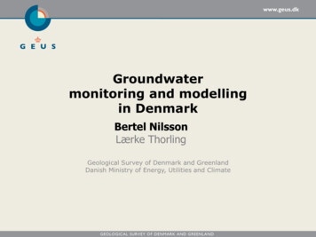
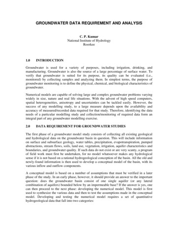
ground-water-quality monitoring program also is affected by the time scale of changes inthe source area for the chemical constituents of interest.4.0PROCESSING OF GROUNDWATER DATABefore any conclusions can be drawn about the cause, extent, and severity of an area’sgroundwater related problems, the raw groundwater data on water levels and water qualityhave to be processed. They then have to be related to the geology and hydrogeology of thearea. The results, presented in graphs, maps, and cross-sections, will enable a diagnosis ofthe problems to be made. We shall assume that such basic maps as topographic, geological,and pedological maps are available.The following graphs and maps have to be prepared that are discussed hereunder: Groundwater hydrographs;Water table-contour map;Depth-to-water table map;Water table-fluctuation map;Head-differences map;Groundwater-quality map.It must be emphasized that a proper interpretation of groundwater data, hydrographs, andmaps requires a coordinate study of a region’s geology, soils, topography, climate,hydrology, land use, and vegetation. If the groundwater conditions in irrigated areas are tobe properly understood and interpreted, cropping patterns, water distribution and supply,and irrigation efficiencies should be known too.Hydrological Information System (HIS) developed under Hydrology Project provides easyaccess to the different variety of data. The monitoring data are systematically organized inthe HIS data base, including: well inventoryexploratory drillingpumping test dataloggingwater levelwater qualityrainfall datameteorological dataGroundwater HydrographsWhen the amount of groundwater in storage increases, the water table rises; when itdecreases, the water table falls. This response of the water table to changes in storage canbe plotted in a hydrograph (Figure 1). Groundwater hydrographs show the water-levelreadings, converted to water levels below ground surface, against their corresponding time.

A hydrograph should be plotted for each observation well or piezometer. It is important toknow the rate of rise of the water table, and even more important, that of its fall. If thegroundwater is not being recharged, the fall of the water table will depend on:- The transmissivity of the water-transmitting layer, KH;- The storativity of this layer, S;- The hydraulic gradient, dh/dx.Figure 1:Hydrograph of a Water Table Observation WellAfter a period of rain (or irrigation) and an initial rise in groundwater levels, they thendecline, rapidly at first, and then more slowly as time passes because both the hydraulicgradient and the transmissivity decrease. The graphical representation of the water tabledecline is known as the natural recession curve. It can be shown that the logarithm of thewater table height decreases linearly with time. Hence, a plot of the water table heightagainst time on semi-logarithmic paper gives a straight line. Groundwater recession curvesare useful in studying changes in groundwater storage and in predicting future groundwaterlevels.The groundwater hydrographs of all the observation points should be systematicallyanalyzed. A comparison of these hydrographs enables us to distinguish different groups ofobservation wells. Each well, belonging to a certain group, shows a similar response to therecharge and discharge pattern of the area. By a similar response, we mean that the waterlevel in these wells starts rising at the same time, attains its maximum value at the sametime, and, after recession starts, reaches its minimum value at the same time. The amplitudeof the water level fluctuation in the various wells need not necessarily be exactly the same,

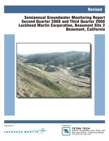
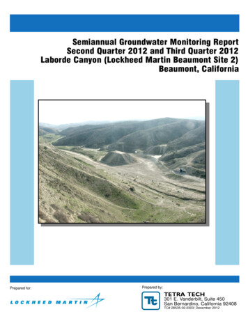
but should show a great similarity. Areas where such wells are sited can then be regarded ashydrological units (i.e. sub-areas in which the watertable reacts to recharge and dischargeeverywhere in the same way).Groundwater hydrographs also offer a means of estimating the annual groundwaterrecharge from rainfall. This, however, requires several years of records on rainfall andwater tables. An average relationship between the two can be established by plotting theannual rise in water table against the annual rainfall (Figure 2). Extending the straight lineuntil it intersects the abscissa gives the amount of rainfall below which there is no rechargeof the groundwater. Any quantity less then this amount is lost by surface runoff andevapotranspiration.Figure 2:Relationship between Annual Groundwater Recharge and RainfallWater Table-Contour MapA water table-contour map shows the elevation and configuration of the water table on acertain date. To construct it, we first have to convert the water-level data from the form ofdepth below surface to the form of water table elevation ( water level height above adatum plane, e.g. mean sea level). These data are then plotted on a topographic base map

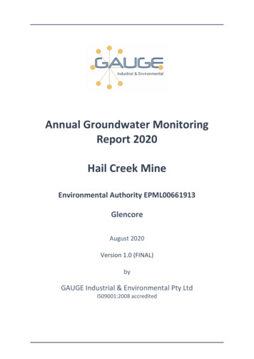
and lines of equal water table elevation are drawn. A proper contour interval should bechosen, depending on the slope of the water table. For a flat water table, 0.25 to 0.50 m maysuit; in steep water table areas, intervals of 1 to 5 m or even more may be needed to avoidovercrowding the map with contour lines. The topographic base map should containcontour lines of the land surface and should show all natural drainage channels and openwater bodies. For the given date, the water levels of these surface waters should also beplotted on the map. Only with these data and data on the land surface elevation can watertable contour lines be drawn correctly (Figure 3).Figure 3:Example of Water Table-Contour LinesTo draw the water table-contour lines, we have to interpolate the water levels between theobservation points, using the linear interpolation method. Instead of preparing the map for acertain date, we could also select a period (e.g. a season or a whole year) and calculate themean water table elevation of each well for that period. This has the advantage ofsmoothing out local or occasional anomalies in water levels. A water table-contour map isan important tool in groundwater investigations because, from it, one can derive thegradient of the water table (dh/dx) and the direction of groundwater flow, which isperpendicular to the water table-contour lines.For a proper interpretation of a water table-contour map, one has to consider not only thetopography, natural drainage pattern, and local recharge and discharge patterns, but also thesubsurface geology. More specifically, one should know the spatial distribution ofpermeable and less permeable layers below the water table. For instance, a clay lensimpedes the downward flow of excess irrigation water or, if the area is not irrigated, thedownward flow of excess rainfall. A groundwater mound will form above such a horizontalbarrier (Figure 4).

Figure 4:A Clay Lens under an Irrigated Area impedes the Downward Flow ofExcess Irrigation WaterWater table-contour maps are graphic representations of the hydraulic gradient of the watertable. The velocity of groundwater flow (v) varies directly with the hydraulic gradient(dh/dx) and, at constant flow velocity, the gradient is inversely related to the hydraulicconductivity (K), or v -K(dh/dx) (Darcy's law). This is a fundamental law governing theinterpretation of hydraulic gradients of water tables. Suppose the flow velocity in two crosssections of equal depth and width is the same, but one cross-section shows a greaterhydraulic gradient than the other, then its hydraulic conductivity must be lower. Asteepening of the hydraulic gradient may thus be found at the boundary of fine-textured andcoarse-textured material, or at a fault where the thickness of the waterbearing layerschanges abruptly.Depth-to-Water Table MapA depth-to-water table map or isobath map, as these names imply, shows the spatialdistribution of the depth of the water table below the land surface. It can be prepared in twoways. The water level data from all the observation wells for a certain date should first beconverted to water levels below land surface (the reference point from which the readingswere taken needs not necessarily to be the land surface). One plots then the transformeddata on the topographical base map near each observation point and draws isobaths or linesof equal depth to groundwater. A suitable contour interval may be 50 cm (Boonstra, 1988).Another way of preparing an isobath map is made by superimposing a water table contourmap for a special date on the topographical map showing contour lines of the land surface.From the two families of contour lines, read the differences in elevation at contourintersections, plot these data on a clean topographical map and draw the isobaths.According to the observation results for a year, the map drawn using the highest water tablelevels indicates the highest water table levels for a year in irrigated lands. The regions ofmap where the groundwater level is between 0-2 m depicts the area having drainageproblems. On the other hand, based on measurement results for a year, the map drawn using

the lowest water table levels indicates to which extent the groundwater falls in a year inirrigated area. The section where the water table level is between 0-1 m determines theareas in which groundwater exists in the root-zone throughout a year. In these areas, farmdrainage systems also need to be established. The map drawn based on water tablemeasurements done in the month of most intensive irrigation indicates to which extentirrigation activities influence the water table. Due to most intensive month in terms ofirrigation application differ from one irrigation scheme to another, this month is defined asmonth in which most of water is released to the system.A variety of factors must be considered if one is to interpret a depth-to-groundwater orisobath map properly. Shallow water tables may occur temporarily, which means that thenatural groundwater runoff cannot cope with an incidental precipitation surplus or irrigationpercolation. They may occur (almost) permanently because the inflow of groundwaterexceeds the outflow, or groundwater outflow is lacking as in topographic depressions. Thedepth and shape of the first impermeable layer below the water table strongly affect theheight of the water table. To explain differences and variations in the depth to water table,one has to consider topography, surface and subsurface geology, climate, direction and rateof groundwater flow, land use, vegetation, irrigation, and the abstraction of groundwater bywells.Water Table-Fluctuation MapA water table-fluctuation map is a map that shows the magnitude and spatial distribution ofthe change in water table over a period (e.g. a whole hydrological year). Using such graphs,we calculate the difference between the highest and the lowest water table height (orpreferably the difference between the mean highest and the mean lowest water table heightfor the two seasons). We then plot these data on a topographic base map and draw lines ofequal change in water table, using a convenient contour interval. A water table-fluctuationmap is a useful tool in the interpretation of drainage problems in areas with large watertable fluctuations, or in areas with poor natural drainage (or upward seepage) andpermanently high water tables (i.e. areas with minor water table fluctuations).The water table in topographic highs is usually deep, whereas in topographic lows it isshallow. This means that on topographic highs there is sufficient space for the water table tochange. This space is lacking in topographic lows where the water table is often close to thesurface. Water table fluctuations are therefore closely related to depth to groundwater.Another factor to consider in interpreting water table-fluctuation maps is the drainable porespace of the soil. The change in water table in fine-textured soils will differ from that incoarse-textured soils, for the same recharge or discharge.Head-Differences MapA head-differences map is a map that shows the magnitude and spatial distribution of thedifferences in hydraulic head between two different soil layers. We calculate the differencein water level between the two piezometers, and plot the result on a map. After choosing aproper contour interval (e.g. 0.10 or 0.20 m), we draw lines of equal head difference.

Another way of drawing such a map is to superimpose a water table-contour map on acontour map of the piezometric surface of the underlying layer. We then read the headdifferences at contour line intersections, plot these on a base map, and draw lines of equalhead difference. The map is a useful tool in estimating upward or downward seepage.The difference in hydraulic head between the shallow and the deep groundwater is directlyrelated to the hydraulic resistance of the low-permeable layer(s). Because such layers areseldom homogeneous and equally thick throughout an area, the hydraulic resistance ofthese layers varies from one place to another. Consequently, the head difference betweenshallow and deep groundwater varies. Local ‘leaks’ in low-permeable layers may result inanomalous differences in hydraulic heads. The hydraulic resistance is especially of interestwhen one is defining upward seepage or natural drainage or the possibilities for tubewelldrainage.Groundwater-Quality MapA groundwater-quality or electrical-conductivity map is a map that shows the magnitudeand spatial variation in the salinity of the groundwater. The EC values of all representativewells (or piezometers) are used for this purpose. Groundwater salinity varies not onlyhorizontally but also vertically; a zonation of groundwater salinity is common in manyareas (e.g. in delta and coastal plains, and in arid plains). It is therefore advisable to preparean electrical-conductivity map not only for the shallow groundwater but also for the deepgroundwater.In electrical conductivity maps, critic

groundwater movement, and the location of recharge and discharge areas, a network of observation wells and/or piezometers has to be established. The objectives of the groundwater level monitoring are to: detect impact of groundwater recharge and abstractions, monitor the groundwater level changes, assess depth to water level,