Transcription
DYNAMIC AIRLINE PRICING AND SEAT AVAILABILITYByKevin R. WilliamsAugust 2017Updated February 2018COWLES FOUNDATION DISCUSSION PAPER NO. 3003UCOWLES FOUNDATION FOR RESEARCH IN ECONOMICSYALE UNIVERSITYBox 208281New Haven, Connecticut 06520-8281http://cowles.yale.edu/
DYNAMIC AIRLINE PRICING AND SEAT AVAILABILITYKevin R. WilliamsSchool of ManagementYale University February 2018†AbstractAirfares are determined by both intertemporal price discrimination and dynamicadjustment to stochastic demand. I estimate a model of dynamic airline pricingaccounting for both forces with new flight-level data. With model estimates, I disentangle key interactions between the arrival pattern of consumer types and remainingcapacity under stochastic demand. I show that the forces are complements in airlinemarkets and lead to significantly higher revenues, as well as increased consumer surplus, compared to a more restrictive pricing regime. Finally, I show that abstractingfrom stochastic demand leads to a systematic bias in estimating demand elasticities.JEL: L11, L12, L93 kevin.williams@yale.eduThis paper is an updated chapter of my dissertation at the University of Minnesota. I thank Tom Holmes,Jim Dana, Aniko Öry, Amil Petrin, Tom Quan and Joel Waldfogel for comments. I thank the seminarparticipants at the Federal Reserve Bank of Minneapolis, Yale School of Management, University of Chicago- Booth, Georgetown University, University of British Columbia, University of Rochester - Simon, DartmouthUniversity, Northwestern University - Kellogg, Federal Reserve Board, Federal Reserve Bank of Richmond,Indiana University, Indiana University - Kelley, Marketing Science, and the Stanford Institute for TheoreticalEconomics (SITE). I also thank the Minnesota Supercomputing Institute (MSI) for providing computationalresources.†
1IntroductionAir Asia (2013) on intertemporal price discrimination:Want cheap fares, book early. If you book your tickets late, chances are you are desperate to fly andtherefore don’t mind paying a little more.1easyJet (2003) on dynamic adjustment to stochastic demand:Our booking system continually reviews bookings for all future flights and tries to predict how populareach flight is likely to be. If the rate at which seats are selling is higher than normal, then the price wouldgo up. This way we avoid the undesirable situation of selling out popular flights months in advance.2Airlines tend to charge high prices to passengers who search for tickets close to theirdate of travel. The conventional view is that these are business travelers and that airlinescapture their high willingness to pay through intertemporal price discrimination. Airlinesalso adjust prices on a day-to-day basis, as capacity is limited and the future demand forany given flight is uncertain. They may adjust fares upward to avoid selling out flightsin advance, or fares may actually fall from one day to the next, after a sequence of lowdemand realizations.This paper examines pricing in the airline industry, taking into account both forces:intertemporal price discrimination (fares responding to time) and dynamic adjustment tostochastic demand (fares responding to seats sold). Collectively, I call this dynamic airlinepricing. I use a new flight-level data set consisting of daily fares and seat availabilitiesto estimate a model of dynamic airline pricing in which firms face a stochastic arrival ofconsumers. The mix of consumer types – business and leisure travelers – is allowed tochange over time, and in the estimated model, late-arriving consumers are significantlymore price-inelastic than early-arriving consumers. I use the model to quantify the welfareeffects of dynamic airline pricing, but also to establish important interactions between intertemporal price discrimination and dynamic adjustment to stochastic demand in airline1Accessed through AirAsia.com’s Investor Relations page entitled, “What is low cost?"Appeared on easyjet.com’s FAQs. Accessed through “Low-Cost Carriers and Low Fares" and “OnlineMarketing: A Customer-Led Approach."21
markets. Finally, I show that analyzing both forces together is critical to quantifying thewelfare implications of airline pricing.The existing research documents the importance of intertemporal price discriminationand dynamic adjustment to stochastic demand separately in airline markets, and thecentral contribution of this paper is to study them jointly and quantify their interactions.Consistent with the idea of market segmentation, Puller, Sengupta, and Wiggins (2015)find that ticket characteristics, such as advance purchase discount (APD) requirements,explain much of the dispersion in fares. Lazarev (2013) quantifies the welfare effectsof airline pricing by estimating a model of intertemporal price discrimination but notdynamic adjustment. He finds a substantial role for this force.3 Escobari (2012) andAlderighi, Nicolini, and Piga (2015) find evidence that airlines face stochastic demand andthat prices respond to remaining capacity. These results support the theoretical predictionsof Gallego and Van Ryzin (1994) and a large branch of research in operations managementthat studies optimal pricing under uncertain demand, limited capacity, and limited timeto sell.4 Indeed, this research has been used to inform airline pricing algorithms.The estimated structural model allows me establish two key points about the interaction between the pricing forces. First, dynamic adjustment complements intertemporalprice discrimination in the airline industry. This is due to the fact that price-inelastic consumers (i.e., business travelers) tend to buy tickets close to the departure date. To be able toprice discriminate towards these late-arriving consumers, airlines must successfully saveseats until close to their departure date. These consumers are then charged high prices.I show that dynamic pricing more efficiently allocates capacity and increases consumerwelfare in the monopoly markets I study relative to either uniform pricing or a pricing3Intertemporal price discrimination can be found in many markets, including video games (Nair 2007),Broadway theater (Leslie 2004), and concerts (Courty and Pagliero 2012). Lambrecht et. al. (2012) provide anoverview of empirical work on price discrimination more broadly.4An overview of the dynamic pricing literature can be found in Elmaghraby and Keskinocak (2003) andTalluri and Van Ryzin (2005). Sweeting (2012) analyzes ticket resale markets. Pashigian and Bowen (1991) andSoysal and Krishnamurthi (2012) study clearance sales and seasonal goods, respectively. Zhao and Zheng(2000), Su (2007), and Dilme and Li (2016) discuss extensions to dynamic pricing models, including consumerdynamics. Seat inventory control has also been studied; see Dana (1999).2
system in which fares vary with only the purchase time but not with past demand shocks.Second, I show that in order to quantify the welfare effects of price discrimination in airlinemarkets, it is necessary to take stochastic demand into account. When abstracting fromstochastic demand, the opportunity cost of selling a seat is the same regardless of the dateof purchase. In reality, the opportunity costs tend to increase in airline markets becauseof the late arrival of price insensitive consumers. As a consequence, I show an empirical procedure abstracting from this feature of the market will systematically overstateconsumers’ price insensitivity. The bias is large close to the departure date.In order to investigate dynamic airline pricing, a detailed data set of ticket purchases isrequired. However, the standard airline data sets used in economic studies (e.g., Goolsbeeand Syverson (2008); Gerardi and Shapiro (2009); Berry and Jia (2010)) are either at themonthly or the quarterly level. Recent papers use new data to get to the flight level.McAfee and Te Velde (2006) and Lazarev (2013) create data sets containing high-frequencyfares. Other papers have obtained high frequency fares as well as a measure of seatssold. Puller, Sengupta, and Wiggins (2015) capture a fraction of sales through a singlecomputer reservation system used by airlines. Escobari (2012) and Clark and Vincent(2012) collect fare and flight availability data, with the available number of seats derivedfrom publicly available seat maps. I use a new data source that allows me to capturethe same information that travel agents see, such as which seats are blocked, occupied,and available. I merge these data with daily fares and flight availability data. In total, Itrack over 1,300 flights in US monopoly markets over a six-month period. I use the datato provide descriptive evidence of both intertemporal price discrimination and dynamicadjustment to stochastic demand.While empirical evidence is informative, it cannot be used to disentangle the interactions between the pricing forces. I proceed by estimating a structural model that containsthree key ingredients: (i) a monopolist has fixed capacity and finite time to sell; (ii) thefirm faces a stochastic arrival of consumers; and (iii) the mix of consumers, correspond-3
ing to business and leisure travelers, is allowed to change over time.5 The firm solves astochastic dynamic programming problem, offering a fare to consumers each day beforedeparture. For the demand system, I assume that a stochastic process brings consumersto the market. The consumers that arrive know when they want to travel and solve astatic discrete choice problem.6 The demand model differs from earlier theoretical work,including Gale and Holmes (1993), and from empirical work such as Lazarev (2013), inwhich consumers are uncertain, and waiting provides more information. In my model theonly reason to wait is to bet on price, and since prices tend to increase, I show that onlya small transaction cost is needed to persuade consumers to decide whether to travel inthe period they arrive. I also provide empirical evidence that suggests this is a reasonableassumption.7 I use the firm’s pricing decision, along with the realizations of demand, toseparately identify the arrival process of consumers and the demand elasticity over time.Using the model estimates, I conduct a series of counterfactual exercises to quantify thewelfare implications of dynamic airline pricing and to highlight how these results dependon the arrival process of consumers. The general finding is that, while more-restrictivepricing systems reduce the ability of firms to price discriminate, the aggregate consumerwelfare gains are limited, or even negative, due to inefficient capacity allocation. That is,while airlines do price discriminate, which we may think only harms consumers, theirpricing also more efficiently allocates scarce seats. In fact, under uniform pricing, revenuesdrop by 2%, but aggregate consumer welfare is unchanged. In this counterfactual, leisureconsumers are charged relatively higher prices, and while business consumers are chargedrelatively lower prices, many flights sell out in advance. Moreover, I find total consumerwelfare is lowered when fares are allowed to respond to the date of purchase but not to thescarcity of seats. However, the pricing forces interact differently under alternative arrival5McAfee and Te Velde (2006) note that stochastic demand models that do not incorporate changes inwillingness to pay over time do not match the positive trend in airfares as the departure date approaches.6The specification is similar to that in Talluri and Van Ryzin (2004) and Vulcano, van Ryzin, and Chaar(2010); however, my model also allows for the mix of consumers to change across time.7Li, Granados, and Netessine (2014) study dynamic consumer behavior in airline markets. Depending onthe specification, they find that between 5% and 20% of consumers are dynamic.4
processes. If price-insensitive consumers were the first to arrive, for example, dynamicadjustment no longer complements intertemporal price discrimination, and stochasticdemand pricing is used to clear excess capacity. This is consistent with fire sales that arecommonly used in retailing.2DataI create an original data set of airfares and seat availabilities with data collected from twopopular online travel services. The first is a travel search engine, owned by Kayak.com,from which I collect daily fares at the itinerary level, with itinerary defined as a routing,airline, flight number(s), and departure date(s) combination. I obtain all one-way andround-trip itinerary fares for stays of less than eight days. The fares recorded correspondto the cheapest ticket available for purchase. The fare data include the fare class and farebasis code, which provide some information regarding the restrictions of the ticket, suchas advance purchase discount requirements.8The second web service, operated by Expertflyer.com, allows users to look up flightavailability. I collect two sources of information. First, I obtain airline seat maps for eachflight. By comparing seat maps across time, I obtain daily bookings. Second, I collect thefare availability (sometimes called fare buckets) for each flight. This information providescensored information regarding which fares are available to purchase. For example, Y9indicates that the Y class fare, which is typically the most expensive coach fare available,has at least nine tickets available for purchase.9 In total, the sample contains 1,362 flightdepartures, with each flight tracked for 60 days. All flights in my data set departed8G21JN5 is an example. This fare basis code indicates a G fare class ticket, and a 21-day advance purchasediscount. Lazarev (2013) has a nice discussion of airline pricing and provides additional details on farerestrictions. Like Lazarev (2013), I model only the pricing choice and not the decision to assign restrictions orquantities for each price.9Regarding the example of the fare basis code G21JN5, the fare availability data might say G5. This meansfive seats remain for that particular fare. Fare availabilities can change because of ticket purchases, but alsobecause of changes input by managers. Both of these potentially result in changes in price, which is the focusof this paper.5
between March 2012 and September 2012.In the following subsections, I discuss route selection (Section 2.1) and the use of seatmaps to infer bookings (Section 2.2), and I provide summary statistics and preliminaryevidence from the data (Section 2.3).2.1Route SelectionI select markets in which to study using the publicly available DB1B tables, which arefrequently used to study airline markets. The DB1B tables contain 10% of domestic ticketpurchases and are at the quarterly level. The data contain neither the date flown nor thepurchase date. I define a market in the DB1B as an origin, destination, quarter. I singleout markets where:(i) there is only one carrier operating;(ii) there is no nearby alternative airport;(iii) at least 95% of flight traffic is not connecting to other cities;(iv) total quarterly traffic is greater than 3,000 passengers;(v) total quarterly traffic is less than 30,000 passengers; and(vi) there is high nonstop traffic.Criteria (i) and (ii) narrow the focus to monopoly markets. One potential complication with using airline seat maps to recover bookings is that it is not clear what fare toassign to an observed change in a seat map. Since airlines offer extensive networks, thedisappearance of a single seat could be associated with one of several thousand possibleitineraries. This is an important consideration since pricing may be different across routes,and this is especially true with regard to feeder routes versus main routes. This issueis addressed in (iii), which essentially rules out most routes from major hubs. Criterion(iv) corresponds to routes with a less than 75% load factor (seats occupied / capacity) ofa daily 50-seat aircraft. This criterion removes routes with irregular service. Criterion (v)6
removes most routes with several daily frequencies. I then look for routes with (vi) highnonstop traffic. This criterion is important for establishing the relevant outside option inthe demand model. In the data, (vi) is negatively correlated with distance (ρ .5). Citieswith very high nonstop traffic percentages tend to be short-distance flights, and, givensuch short distances, many consumers may choose to drive instead. At the same time, theDB1B data suggest that longer flights have lower nonstop traffic percentages, suggestingthat more consumers choose a connecting flight option.I select four city pairs, or eight directional routings, given the selection criteria above.All directional routings either originate or end in Boston, MA. The other cities are: SanDiego, CA; Austin, TX; Kansas City, MO; and Jacksonville, FL. The selected markets haveclose to 100% direct traffic, meaning that very few passengers connect to other cities.The percent of nonstop traffic ranges between 40% and 70%. Three of the four city pairsare operated by JetBlue and the other by Delta Air Lines.10 The selected markets are alllow-frequency, with at most two daily frequencies.Three other features of the data are worth noting. First, JetBlue prices itineraries at thesegment level; that is, consumers wishing to purchase round-trip tickets on this carrierpurchase two one-way tickets. As a consequence, round-trip fares in these markets areexactly equal to the sum of the corresponding one-way fares. Since fares must be attributedto each seat map change, this feature of the data makes it easier to justify the fare involved.Second, JetBlue does not oversell flights, while most other air carriers do.11 I will use thisfeature of the data to simplify the pricing problem in the next section. Third, JetBlue doesnot offer first class on the routes studied. This allows for investigating all sales and alsocontrols for one aspect of versioning (first class versus economy class).1210At the time of data collection, flights between Kansas City and Boston were operated by regional carrierson behalf of Delta Air Lines. Since Delta Air Lines determines the fares for this market, I collectively call theseregional carriers Delta.11In the legal section of the JetBlue website, under Passenger Service Plan: “JetBlue does not overbookflights. However some situations, such as flight cancellations and reaccommodation, might create a similarsituation."12The Delta first class cabins were typically six seats for the market studied.7
2.2Inference and Accuracy of Seat MapsA seat map is a graphical representation of occupied and unoccupied seats for a givenflight at a select point in time before the departure date. Many airlines that have assignedseating present seat maps to consumers during the booking process. When a consumerbooks a ticket and selects a seat, the seat map changes to reflect that an unoccupied seat isnow occupied. The next consumer wishing to purchase a ticket on the flight is offered anupdated seat map and can choose one of the remaining unoccupied seats. By differencingseat maps across time – in this case daily – inferences can be made about daily bookings.I use a new data source that allows me to distinguish between various types of occupiedand occupied seats.Figure 1 presents a sample seat map: occupied seats are in solid blue, while theunshaded blocks correspond to unoccupied seats. Seats with a "P" are available, butclassified as premium. These seats are located toward the front of the aircraft or in exitrows. Some airlines charge a premium to be seated in these rows. Finally, the seat mapindicates seats currently blocked by the airline with "X"s. Seats that are blocked are usuallynot disclosed on airline websites; however, I am able to capture these data through theweb service used. Seats may be blocked due to crew rest, weight and balance, because aseat is broken, or because the airline reserves accessible seats for handicapped passengersuntil the day of departure.13 For every seat map collected, I aggregate the number ofoccupied, unoccupied, and blocked seats. I compare the aggregate counts across days todetermine bookings by day prior to departure.13Seat blocking may be used to encourage consumers to purchase tickets or upgrade, as they give theimpression that the cabin is closer to capacity. However, the data suggest that airlines predominantly blockseats in exit rows and at the front and/or back of the cabin until closer to the departure date or when bookingsdemand additional seats. 69% of the flights in the sample experience changes in the number of blocked seats,and while I do not model the decision to block/unblock seats, I do take this information into account whendetermining bookings. Knowing which seats are blocked is important because it allows me to distinguishbetween consumers’ decisions and airlines’ adjustment of the supply of seats. For example, if an airlineunblocks six seats, without these data, I would erroneously conclude that six passengers canceled theirtickets.8
Figure 1:An example seat map. The white blocks are unoccupied seats, the blue blocks are occupied, the blocks withthe X’s are blocked seats, and the blocks with a "P" are premium, unoccupied seats.Unfortunately, seat maps may not be accurate representations of true flight loads. Thisis especially problematic if consumers do not select seats at the time of booking. Thismeasurement error would systematically understate sales early on, but then overstatelast-minute sales when consumers without existing seat assignments are assigned seats.From a modeling perspective, this measurement error would lead to an overstatement9
of the arrival of business consumers. Ideally, the severity of measurement error of mydata could be assessed by matching changes in seat maps with bookings, however this isimpossible with the publicly available data. While both imperfect, I perform two analysesto gauge the magnitude of the measurement error in using seat maps.First, I match monthly enplanements using my seat maps aggregated on the the day ofdeparture with actual monthly enplanements reported in the T100 Segment tables. Thesetables record the total number of monthly enplanements by airline and route. Figure 2provides a scatter plot that compares the two statistics. All the points closely follow the45-degree line and I find seat maps differ with true enplanements by less than two percenton average. However, what really matters is the difference between actual loads andseat maps at the flight-day before departure level. Unfortunately, this analysis cannot beperformed with the collected data set.Figure 2: Estimated Seat Map Measurement Error at the Monthly-LevelNote: Measurement error estimated by comparing monthly enplanements using the T100 Tables and aggregating seat mapsto the monthly level. The solid line reflects zero measurement error. The black-squares correspond to Delta observations.The two outliers are due to a change in flight numbers which were not picked up by the data collection process in onemonth.10
Second, I create a new data set that allows me to estimate the measurement error at theflight-day before departure level. The mobile website version of United.com allows usersto examine seat maps for upcoming flights. In addition, for premium cabins, the airlinealso reports the number of consumers booked into the cabin. I randomly select flights,departure dates, and search dates, and, in total, I obtain 15,567 observations. With thesedata I find that seat maps understate reported load factor by 2.3% on average (around1-2 seats). Figure 3 plots the average measurement error by day before departure (t 60corresponds to the day that flights leave), as well as a polynomial smooth of the data. Ifind the difference to range between 0% to 5% across days. Two caveats are worth noting.First, I cannot reject that the measurement error is constant across days. Seat maps aremost accurate far in advance (60 to 40 days out) and close to the departure date. Second,while these data do not indicate all blocked seats and the main sample does, they are fora different airline, different markets, and for a different cabin.Figure 3: Estimated Seat Map Measurement Error by Day Before DepartureNote: Measurement error estimated by comparing seat maps with reported load factor using the United Airlines mobilewebsite. The dots correspond to the daily mean, and the line corresponds to fitted values of an orthogonal polynomialregression of the fourth degree. Total sample size is equal to 15,567 with an average load factor of 70.7%.11
2.3Summary Statistics and Preliminary EvidenceSummary statistics for the data sample appear in Table 1. The average one-way ticketin my sample is 283, whereas the average round-trip fare is 528. The discrepancy inone-way and round-trip fares can be attributed to the flights operated by Delta since Deltadoes not price at the segment level, but JetBlue does.Table 1: Summary Statistics for the Data SampleVariableMeanStd. Dev.Median5th pctile95th pctile282.778117.788272.800129.800498.800Load Factor0.8490.0770.8670.6880.933Daily Booking Rate0.7711.6000.0000.0004.000Daily Fare Change ( )3.17036.3980.000-30.00060.000Unique Fares (per itin.)6.7932.1967.0003.00010.000Oneway Fare ( )Note: Summary statistics for 1,362 flights tracked between 3/2/2012 and 8/24/2012. The total numberof observations is 79,856. Load Factor is reported between zero and one the day of departure. Thedaily booking rate and fare change differences across search days within flights. Finally, unique faresis at the itinerary level and denotes the number of unique price points per flight.Reported load factor is the number of occupied seats divided by capacity on the dayflights leave, and is reported between 0 and 1. In my sample, the average load factor is85%, ranging from 77% to 89% by market. The booking rate corresponds to the meandifference in occupied seats across consecutive days. I find the average booking rate tobe 0.78 seats per day, per flight. At the 5th percentile, zero seats per flight are booked aday, and at the 95th percentile, four seats per flight are booked a day. Airline markets areassociated with low daily demand, as 57% of the seat maps in the sample do not changeacross consecutive days. The fare change rate is an indicator variable equal to one if theitinerary fare changes across consecutive days. I find the daily rate of fare changes to be20%, so that the itineraries in my sample typically change price 12 times in 60 days. Onaverage, each itinerary reaches 6.8 unique fares, and given that the average itinerary sees12
12 fare changes, on average, this implies that fares usually fluctuate up and down usuallyseveral times within 60 days. I use the institutional feature that fares are chosen from adiscrete set (fare buckets) in the model.Figure 4: Frequency and Magnitude of Fare Changes by Day Before DepartureNote: The top panel shows the percent of itineraries which see fares increase or decrease by day before departure. Thelower panel plots the magnitude of the fare declines and increases by day before departure. The vertical lines correspondto advance-purchase discount periods (fare fences).Figure 4 shows the frequency and magnitude of fare changes across time. The toppanel indicates the fraction of itineraries that experience fare hikes versus fare discountsby day before departure, and the bottom panel indicates the magnitude of these farechanges (i.e., a plot of first differences, conditional on the direction of the fare change). Forexample, in the left plot, 40 days prior to departure (t 20), roughly 10% of fares increaseand 10% of fares decrease. The remaining 80% of fares are held constant. Moving tothe bottom panel, the magnitude of fare increases and declines 40 days out is roughly 50. The top panel confirms fares change throughout time, and this is also true for faredeclines. Note that well before the departure date, the number of fare hikes and declinesis roughly even. The fraction of itineraries that experience fare hikes increases over time.13
There are four noticeable jumps in the line, indicating fare hikes. These jumps correspondto crossing three, seven, 14 and 21 days prior to departure, or when the advance purchasediscounts placed on many tickets expire.14 The use of advance purchase discounts (APDs)is consistent with the story of intertemporal price discrimination. Surprisingly, though,the use of APDs is not universal. Only 20% of itineraries experience fare hikes at 21 days,and less than 50% increase at 14 days. Just under 70% of itineraries see an increase in farewhen crossing the seven-day APD requirement.Figure 5: Mean Fare and Load Factor by Day Before DepartureNote: Average fare and load factor by day before departure. Includes all oneway observations in the data sample. Thevertical lines correspond to advance-purchase discount periods (fare fences).Moving to statistics in levels, Figure 5 plots the mean fare and mean load factor (seatsoccupied/capacity) by day before departure. The plot confirms that the overall trend inprices is positive, with fares increasing from roughly 225 to over 425 in sixty days.The noticeable jumps in the fare time series occur when crossing the APD fences notedin Figure 4. At 60 days prior to departure, roughly 40% of seats are already occupied.Consequently, I observe about half the bookings on any given flight. The booking curve14Advance purchase discounts are sometimes placed at four, ten, and 30 days prior to departure, but this isnot the case for the data I collect.14
for flights in the sample is smooth across time, leveling off at 85% roughly three days priorto departure. The fact that fares tend to double but that consumers still purchase tickets issuggestive evidence that consumers of different types purchase tickets towards the dateof travel.Table 2: Dynamic Substitution Regressions(1)-0.231 (0.042)(2)-0.223 (0.042)(3)-0.220 (0.042)A
School of Management Yale University February 2018y Abstract Airfares are determined by both intertemporal price discrimination and dynamic adjustment to stochastic demand. I estimate a model of dynamic airline pricing . Airlines tend to charge high prices to passengers who search for tickets close to their date of travel. The conventional .