Transcription
Optimal Pricing and SeatAllocation in Airline IndustryUnder Market CompetitionPhD ThesisOral Exam PresentationSyed Asif Raza
OutlineRevenue Management (RM)¾ Background and Literature¾ Model and Results¾ Conclusion and Future Works¾ Questions¾
Airline RMAirline ScheduleDesign and ne RevenueManagementRevenueManagement issimply thepractice ofmaximisingRevenue fromPerishable assets(seats) through acombination ofPricing &InventorycontrolsStatic SeatInventory ControlSeat InventoryDynamic SeatInventory ControlStatic PricingPricingDynamic Pricing
Missing Connections in AirlineRM StudiesMarketCompetitionIgnoredRevenue tConnectionReservation ControlSeat Inventory ControlFare Class MixSegmentODOverbookingItinerary ControlPoint-of-Sale
Review Articles:¾¾¾¾¾¾McGill and Van Ryzin (1999)- Revenue Management:Research overview and prospects.Pak and Piersma (2002)- Overview of OR techniques inairline RM.Silver (2004)- An overview of heuristic solution methodsBarnhart et al. (2003) – Application of operations researchin the air transport industry.Elmagraby and Keskinocak (2003) -Dynamic pricing in thepresence of inventory considerations: Research overview,current practices, and future directionsBitran and Caldentey (2003)- An overview of pricingmodels for Revenue Management.
Competition in RM¾Cote et al. (2003)- Mathematical optimization approach forintegrated seat allocation and pricing in airline industry.¾¾¾Dai et al. (2005)- Multiple firms competition in RM context.¾¾¾Bi-level mathematical optimization model is presented forjoint determination of fare pricing and seat allocationThe customer demand is considered price insensitive andthe model is non dynamicCompetitive prices are determined for both the deterministicand stochastic price sensitive demand for a known capacity.Mostly the analysis consider duopoly competitionChen et al.(2005) – Newsvendor pricing game¾¾Jointly determined the competitive pricing and capacity forthe competing firms for a single commodityUnique Nash equilibrium is determined analytically
Competition in Airline RM:¾¾¾¾¾Hotelling (1929)-Scheduling decision under competitionBorenstein et al. (2003)- An empirical paper, focus onbroad competition problem but ignore any seat allocation/pricing modeling.Belobaba and Wilson (1997)- Simulation model to studyscheduling strategy under market competition.Lippman and McCardle (1997)- two-firm pricingcompetition.Teodorovic and Krcmar-Nozic (1989)- Multi-criteria modelto determine flight frequencies on an airline network undercompetitive conditions.
Objectives of thesisDevelop new models for jointdetermination of competitive fare pricingand seat allocation in airline Industry¾ Develop new solution methodologies forjoint determination of pricing and capacityin RM¾
Airline RM Competition ModelsAirline RM game is developed mainly induopoly market¾ Two game theoretic models are presented¾ The models are studied for both thecooperative and non-cooperative gamesettings.¾ Numerical analysis with statistical DOE¾
Distribution Free Approach is RM¾ An alternative approach for joint determinationof pricing and capacity under monopoly¾ Determines lower bound (worst possible)revenue estimate¾ The approach is addressed to:¾ Standard Newsvendor problem¾ Extension to Shortage cost Penalty¾ Extension to Shortage and Holding cost¾ Extension to recourse case¾ Extension random yield¾ Extension to multiple items
Competition Models in Airline RM:Π i PLi min{S Li , Bi } PHi min{S Hi , Ci min{S Li , Bi }}, i {1,2}
Modeling ApproachesMultiplicative ModelAdditive ModelSLi D Li ξ Li , i {1,2}SLi D Li ξ Li , i {1,2}SHi D Hi ξ Hi , i {1,2}SHi D Hi ξ Hi , i {1,2}WhereWhereE[ξ Li ] E[ξ Hi ] 0E[ξ Li ] E[ξ Hi ] 1ξ Li [ξ Li , ξ Li ]ξ Li [ξ Li , ξ Li ]ξ Hi [ξ Hi , ξ Hi ]ξ Hi [ξ Hi , ξ Hi ]Both ξ Li and ξ Hi follow Increasing Generalized Failure Rate (IGFR)A Uniform Distribution is assumed
AssumptionsThe Demand is modeled with linear price sensitive determinsitic demand functionsDLi α Li β Li PLi θ Lij PLj , DHi α Hi β Hi PHi θ Hij PHjβ Li θ Lij , β Li ,θ Lij 0, i j , i, j {1,2},β Hi θ Hij , β Hi ,θ Hij 0, i j , i, j {1,2},It is also assumed that D L1 D L1 D H1 D H1 D H1 D L1 0, 0, 0 0, 0, 0 and PL1 PL 2 PH 1 PH 2 PH 1 PH 2 PL1 PL 2
Additive ModelΠ Li PLi Eξ Li [min{S Li , Bi }] PLi Eξ Li [ S Li ] PLi Eξ Li [ S Li Bi ] PLi Bi PLiBi DLi ξ ΦLi(ξ Li ) dξ LiLiΠ Hi Eξ Li Eξ Hi [ PHi min{S Hi , Ci min{S Li , Bi }}]Bi DLiyi PHi Ci Bi Φ Li (ξ Li ) dξ Li Φ Hi (ξ Hi ) dξ Hi ξξLiHi Whereyi Ci Bi DLi ξ ΦLi(ξ Li ) dξ Li DHi BiLiBi DLiΠ i PHi Ci (PHi PLi )Bi (PHi PLi ) ξ ΦLiyi PHi Φ Hi (ξ Hi ) dξ Hiξ HiLi(ξ Li ) dξ Li
Multiplicative ModelΠ i PHi Ci (PHi PLi )Bi (PHi PLi )DLiBi / DLi Φ0 PHi DHiyi / DHi ΦHi(ξ Hi ) dξ Hi0WhereBi / DLiyi Ci Bi DLi Φ Li (ξ Li ) dξ Li0Li(ξ Li ) dξ Li
Game Theory1 DMOptimizationSide PaymentsStaticCooperative 1 DMEnvironmentCertainNo Side PaymentsNonCooperative1 DMOptimal ControlDynamicSide PaymentsCooperative 1 DMNo Side PaymentsNonCooperative
Competition Analysis¾Non-cooperative analysis¾ Uniquenessof Nash Equilibrium (NE)¾ Numerical analysis with a Statistical DesignOf Experiment (s) (DOE).¾Cooperative analysis¾ Bargaininggame with No Side Paymentoptions (NSP)¾ Bargaining game with Side Payment options(SP)
Nash EquilibriumA pair of strategies (x1N , x 2N ) is said to constitute a NashEquilibrium (NE) if the following pair of inequalities are satisfied forall x1 X1 and for all x 2 X 2 :f1 (x1N , x 2N ) f1 (x1 , x 2N ) and f 2 (x1N , x 2N ) f 2 (x1N , x 2 )Where X1 and X 2 represent the strategy sets of player 1 andplayer 2 respectively.For a booking limit pre - commitment 2 Π L1 2 Π L1 Unique Nash equilibrium2 PL1 PL 2 PL1 2 Π H1 2 Π H1 Unique Nash equilibrium2 PH 1 PH 2 PH 1
Nash Bargain SolutionNo Side Payment Option()(Max Π1 Π1NE Π 2 Π 2NESubject toΠ1 Π1NEΠ 2 Π 2NE)With Side Payments OptionMax Π1 Π 2Subject toΠ1 Π1NEΠ 2 Π 2NESide Payments1SP Π1FC Π1NE Π 2NE Π 2FC2()
Numerical AnalysisCi 100, P Li 0, PLi 100, P Hi 100, PHi 200, i {1,2}α Li 60, α Hi 40, β Li 0.25, β Hi 0.15 , i {1,2}θ Lij 0.15, θ Hij 0.10, i, j {1, 2}, i jFor Additive Model[ξ Li , ξ Li ] [ξ Hi , ξ Hi ] [ 30 , 30 ] , i {1, 2}For Multiplica tive Model[ξ Li , ξ Li ] [ξ Hi , ξ Hi ] [ 0 , 2 ] , i {1, 2}
Non-Cooperative Analysis(Symmetric eUniformAirline 172.35176.53205.1813570.21Airline 272.35176.53205.1813570.21Airline 172.89171.47200.0413349.00Airline 272.90171.47200.0413349.00Airline 184.90175.50208.3213608.25Airline 284.90175.50208.3213608.25Airline 185.91171.56200.2613355.13Airline ormNormalLow Fare PriceHigh Fare PricePayoff
Non-Cooperative Analysis(Asymmetric market)ParametersLevelsC2[80 (-), 120 ( )]βL2[0.2 (-), 0.3 ( )]βH2[0.1(-), 0.2 ( )] L21[0.1(-), 0.2 ( )] H21[0.05 (-), 0.15 ( )]Model Type (I)[Additive (-), Multiplicative ( )]
DOE-Non Cooperative Gameˆ 1 14861 598 C2 537 β L 2 1337 β H 2 867θ H 21 922 β H 2θ H 21Πˆ 15234 1182 β 3080 β 1182 θ 2821θ 1724β θΠ2L2H2L 21H 21H 2 H 21Bˆ 76.061 1.329 β 1.019β 5.172 I 0.858β θ1L2H2H 2 H 21Bˆ 2 69.998 10.033 C2 9.677 β H 2θ H 21 7.946 β H 2 I 7.605θ H 21IPˆL1 178.343 6.050 C2 7.156 β L 2 6.256 β H 2 4.449θ L 21 4.882θ H 21Pˆ 169 13.63 C 18.33β 10.83θL22L2L 21PˆH 1 235.63 6.83 C2 23.59 β H 2 13.79 θ H 21 7.99I 18.05β H 2θ H 21Pˆ 273.53 12.85 C 54.36 β 30.74θ 40.48β θH22H2H 21H 2 H 21
Cooperative Analysis (Bargaining Game)AdditiveAirline 1Airline 76.53205.1813570.2172.35176.53205.1813570.21NBS no side BS with sidepaymentsGain Of Cooperation2162.22162.2
Cooperative Analysis (Bargaining Game)MultiplicativeAirline 1Airline 8.2584.90175.50208.3213608.25NBS no side .24NBS with side .24Non-cooperativeGain Of Cooperation1604.001604.00
Comparing NSP with NE¾¾¾Airline 1Revenue improvesabout 5.4%1.9% more seats forHigh fare customersLow and high fareprices increase by4.8% and 35%respectively¾¾¾Airline 2Revenue improves6.5%5.3% more seats forhigh fare classLow and high fareprices increase is9.6% and 28.4%
Comparing SP with NSP¾¾¾Airline 1Revenue improvesabout 6%1.9% more seats forHigh fare customersLow and high fareprices increase by6.7% and 8.6%respectively¾¾¾Airline 2Revenue improves5.2%1.6% more seat tohigh fare class but notsignificant.Low and high fareprices increase is6.3% and 5.8%respectively
Side Payments300Side 0
Newsvendor Problem and RMYao (2002)’ s thesis investigatesnewsvendor problem (NVP) with pricing inthe context of SCM and reported that theelegant structure of the problem also findsapplications in RM.¾ In standard newsvendor problem optimalquantity is determined for a singleperishable asset with stochastic demandhaving an objective to maximize therevenue¾
Proposed Extension to NVPInvestigate alternative solution approachto NVP with pricing using Distribution FreeApproach.¾ Using Distribution Free approach studyseveral extensions to NVP with applicationin RM¾
Distribution Based Vs.Distribution Free Approach¾Distribution manddistributionItmaximizestherevenueunderaknown distribution¾Distribution Free¾¾Modeling requiresonly the mean andstandard errorestimate of thedemand.It maximizes therevenue under theworst possibledemand distribution.
Newsvendor problem withPricingAdditive Model :RD D ξΠ ( P, Q) Eξ [ P min{Q, RD} C Q] ( P C ) Q P Eξ [Q RD] WhereEξ [Q RD] (σ2 (D Q )2)2 1/ 2 (D Q )**Π LB ( PLB, QLB) (PLB C )QLB PLB(σ2 (D QLB )2)2 1/ 2 ( D QLB )
Newsvendor problem withPricingMultiplicative Model :RD D ξΠ ( P, Q) Eξ [ P min{Q, RD} C Q] ( P C ) Q P D Eξ [Q / D ξ ] WhereEξ [Q / D ξ ] (σ 2 (1 Q / D )2)2 1/ 2Π LB ( P , Q ) (PLB C )QLB PLB*LB*LB (1 Q / D )(σD2 (1 Q / D )2)2 1/ 2 (1 Q / D )
Proving concavityΠ LB is quasi concave if, 2 Π LB 2 Π LBi) 0 0,22 QLB PLB 2 Π LB 2 Π LB 2 Π LBii ) H 0 22 PLB QLB PLB QLBFor Additive modelΠ LB is quasi concave; if i ) QLB D, ii ) PLB σ4 D'For Multiplicative modelΠ LB is quasi concave; if i ) D QLB 2 D, ii ) PLB Dσ2 D' (σ 2)
Extension to Holding andShortage cost case:Π ( P , Q ) E ξ [ P min{ Q , RD } C Q G [ Q RD ] S [ RD D ] ] ( P S C ) Q (P S G ) E ξ [ Q RD ] S D**Π LB ( PLB, Q LB) (PLB S C ) Q LB S D (PLB(σ G S)2 (D Q LB )2)2 1/ 2 ( D Q LB )
Proving concavityFor Additive modelΠ LB is quasi concave; if i ) QLB D, ii ) PLB (G S ) σ4 D'For Multiplicative modelΠ LB is quasi concave; if i ) D QLB 2 D, ii ) PLB Dσ (G S )2 D' (σ 2)
Extension to Shortage costcase:Additive Model :RD D ξΠ ( P, Q) Eξ [ P min{Q, RD} C Q S [ RD D] ] ( P S C ) Q (P S ) Eξ [Q RD] S D**Π LB ( PLB, QLB) (PLB S C )QLB S D (PLB(σ S)2 (D QLB )2)2 1/ 2 ( D QLB )Π LB is quasi concave; if i ) QLB D, ii ) PLB S σ4 D'
Recourse case:Additive Model :RD D ξΠ ( P, Q) ( P C Cr ) Q (P Cr ) Eξ [Q RD] Cr D**Π LB ( PLB, QLB) (PLB Cr C )QLB Cr D (PLB(σ C )r2 (D QLB )2)2 1/ 2 ( D QLB )Π LB is quasi concave; if i ) QLB D, ii ) PLB σ4 D'iii ) Cr PLB
Random yield case:Additive Model :RD D ξΠ ( P, Q) Eξ [ P min{G (Q), RD} C Q ] ( ρ P C ) Q P Eξ [G (Q) RD] **Π LB ( PLB, QLB) (ρ PLB C )QLB PLB(σ2 ρ QLB (1 ρ ) (ρ QLB D )2 2 Π LB 0 if ; σ 1 / 2i)2 PLB 2 Π LBDii ) 0 if ; QLB , D is IPE2 QLBρ)2 1/ 2 ( ρ QLB D)
Multiple Product case:nΠ ( P, Q) Eξi [ Pi min{Qi , RDi } Ci Qi ]i 1Subject to :n C Q Bi 1iin()Π LB ( P , Q ) PLBi Ci QLBi PLBi*LB*LBSubject to :n C Qi 1iLBi Bi 1(σ (D Q ) ) (D Q )2i2 1/ 2iLBii2LBi
Numerical AnalysisExperimentation with each extension follows :100 randomly generated problemsC U[20, 100], α U[100, 200], β U[0.05, 0.3]S U[0.1, 0.2] C, G U[0.2, 0.3] C, C r U[1.2, 1.4] Cρ U[0.5, 0.9], B U[10,000,15,000], D α - β PFor additive model, [ξ , ξ ], ξ ξ U(0, 30]For multiplicative model, [ξ , ξ ], ξ ξ U(0, 2]
Standard NewsvendorProblemUniform¾EVAI Improves revenue 0.25%¾13% over-stocking¾0.85% under-pricingAdditive ModelNormal¾EVAI Improves revenue 0.13%¾3% over-stocking¾0.81% under-pricingUniform¾EVAI Improves revenue 0.75%¾0.59% under-stockingMultiplicative Model¾0.01% over-pricingNormal¾EVAI Improves revenue 0.60%¾0.13% over-stocking¾0.30% over-pricing
Extension to Shortage andHolding CostUniform¾EVAI Improves revenue 0.20%¾0.48% under-stockingAdditive Model¾0.89% under-pricingNormal¾EVAI Improves revenue 0.09%¾2.3% over-stocking¾0.85% under-pricingUniform¾EVAI Improves revenue 0.48%¾2.45% under-stockingMultiplicative Model¾0.19% over-pricingNormal¾EVAI Improves revenue 0.38%¾1.68% over-stocking¾0.30% over-pricing
Extension Uniform¾EVAI Improves revenue 0.29%¾0.86% over-stocking¾0.81% under-pricingRecourse CaseNormal¾EVAI Improves revenue 0.17%¾3.5% over-stocking¾0.77% under-pricingUniform¾EVAI Improves revenue 0.42%¾0.53% over-stocking¾0.80% under-pricingRandom Yield CaseNormal¾EVAI Improves revenue 0.22%
¾Bitran and Caldentey (2003)- An overview of pricing models for Revenue Management. . ¾Bi-level mathematical optimization model is presented for joint determination of fare pricing and seat allocation ¾The customer demand is considered price insensitive and the model is non dynamic ¾Dai et al. (2005)- Multiple firms competition in RM context. ¾Competitive prices are determined for both .