Transcription
Active and Passive InvestingNicolae Gârleanu and Lasse Heje Pedersen October 1, 2019AbstractWe model how investors allocate between asset managers, managers choose theirportfolios of multiple securities, fees are set, and security prices are determined. Theoptimal passive portfolio is linked to the “expected market portfolio,” while the optimal active portfolio has elements of value and quality investing. We make preciseSamuelson’s Dictum by showing that macro inefficiency is greater than micro inefficiency under realistic conditions — in fact, all inefficiency arises from systematic factorswhen the number of assets is large. Further, we show how the costs of active and passive investing affect macro and micro efficiency, fees, and assets managed by active andpassive managers. Our findings help explain empirical facts about the rise of delegatedasset management, the composition of passive indices, and the resulting changes infinancial markets.Keywords: asset pricing, market efficiency, asset management, search, informationJEL Codes: D4, D53, D8, G02, G12, G14, G23, L1Gârleanu is at the Haas School of Business, University of California, Berkeley, and NBER; e-mail: garleanu@berkeley.edu. Pedersen is at AQR Capital Management, Copenhagen Business School, New York University, and CEPR; www.lhpedersen.com. We are grateful for helpful comments from Antti Ilmanen, KelvinLee, and Peter Norman Sørensen as well as from seminar participants at the Berkeley-Columbia Meeting inEngineering and Statistics, Federal Reserve Bank of New York, and Copenhagen Business School. Pedersen gratefully acknowledges support from the FRIC Center for Financial Frictions (grant no. DNRF102).AQR Capital Management is a global investment management firm, which may or may not apply similarinvestment techniques or methods of analysis as described herein. The views expressed here are those of theauthors and not necessarily those of AQR.
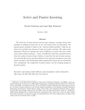
Over the past half century, financial markets have witnessed a continual rise of delegatedasset management and, especially over the past decade, a marked rise of passive management, as seen in Figure 1. This delegation has potentially profound implications for marketefficiency (see, e.g., the presidential addresses to the American Finance Association of Grossman (1995), Stein (2009), and Stambaugh (2014)), investor behavior (presidential address ofGruber (1996)), and asset management fees (e.g., the presidential address of French (2008)).The rise of delegated management raises several questions: What is the optimal portfolioof active (i.e., informed) and passive (i.e., uninformed) managers, respectively? What determines the number of investors choosing active management, passive management, or directholdings? What are the implications of delegated management on market efficiency at themicro and macro levels? How do macro and micro efficiencies depend on the costs of activeand passive management?We address these questions in an asymmetric-information equilibrium model where security prices, asset management fees, portfolio decisions, and investor behavior are jointlydetermined. Our main findings are: (1) the optimal passive portfolio is the “expected marketportfolio,” tilted away from assets with the most supply uncertainty; (2) the optimal activeportfolio has elements of value and quality investing; (3) macro inefficiency is greater thanmicro inefficiency (consistent with Samuelson’s Dictum) when there exists a strong commonfactor in security fundamentals or when the number of securities is large; (4) when information costs decline, the number of active managers increases, active fees decrease, marketinefficiency decreases, especially macro inefficiency (counter to part of Samuelson’s Dictum);(5) when the cost of passive investing decreases, market inefficiency increases, especiallymacro inefficiency, the number of active mangers decreases, and active fees drop by less thanpassive fees; and (6) market inefficiency is linked to the economic value of information andto entropy. These findings help explain a number of empirical findings and give rise to newtests as we discuss below.To understand our results, let us briefly explain the framework. We introduce assetmanagers into the classic noisy-rational-expectations-equilibrium (REE) model of Grossman1
Figure 1: Ownership of US Equities. The figure shows the decline in direct holdings(blue) and the rise of delegated management, including active mutual funds and hedge funds(the two red areas), passive mutual funds and ETFs (the green areas), and pension plansand other equity owners (grey areas). The data is from the Federal Reserve’s Flow of FundsReport, except the hedge fund data, which is from HFR, and the breakdown of mutual fundholdings into active versus passive, which is from Morningstar.and Stiglitz (1980), following Gârleanu and Pedersen (2018). We extend the model to covermultiple securities (in the spirit of Admati (1985), who also considers multiple securities, butnot asset managers) and costly asset management. 1 Having asset managers with multiplesecurities allows us to study portfolio choice and macro vs. micro efficiency and having costlyactive and passive management is essential to study the effects of changes in these costs asinformation technology evolves.Investors must decide whether to invest on their own, allocate to a passive manager,or search for an active manager. Each of these alternatives is associated with a cost: selfdirected trade has an individual-specific cost (time and brokerage fees), passive investinghas a fee (equal to the marginal cost of passive management, in equilibrium), and activeinvesting is associated with a search cost (the cost of finding and vetting a manager toGârleanu and Pedersen (2018) features a single risky security and no passive managers, and assumes thatself-directed trade is costless. See also Garcı́a and Vanden (2009), who considers an alternative generalizationof the noisy rational expectations framework with mutual funds trading a single risky asset. Influential papersfocusing on other aspects of asset management include Berk and Green (2004), Petajisto (2009), Pastor andStambaugh (2012), Vayanos and Woolley (2013), Berk and Binsbergen (2015), and Pastor et al. (2015).12
ensure that she is informed) plus an active management fee. Active and passive managersdetermine which portfolios to choose and, in addition, active managers decide whether ornot to acquire information. Market clearing requires that the total demand for securitiesequals the supply, which is noisy (e.g., because of share issuance, share repurchases, changesin the float, private holdings, etc.).Passive managers seek to choose the best possible portfolio conditional on observed prices(but not conditional on the information that active managers acquire). One may wonderwhether they should choose the “market portfolio” (the market-capitalization weighted portfolio of all assets), which is the standard benchmark in the Capital Asset Pricing Model(CAPM). While the market portfolio is the focal point of much of financial economics, itis not discussed in the context of REE models because supply noise renders it unobservable (likewise, in the real world no one knows the true market portfolio as emphasized byRoll (1977)); furthermore, much of the REE literature studies a single asset, precluding ameaningful analysis of portfolios. Bridging the REE literature and the CAPM, we showthat passive investors choose the closest thing they can get to the market portfolio, namelythe “expected market portfolio” based on the distribution of the supply and what can belearned from public signals, under certain conditions (e.g, i.i.d. shocks across securities).This behavior resembles what real-world passive investors do, namely choosing an indexthat is rebalanced based on public information. However, indices only hold a subset of allsecurities, typically large and mature firms with sufficient time since their initial public offering. In a similar spirit, we show that passive investors optimally over-weight securities withless supply uncertainty in the more general case when shocks are correlated across securitiesvia a factor structure. Hence, our framework presents a first step toward a theory of optimalsecurity indices.Turning to active managers, we show that they use their information advantage in severalways. First, they naturally tend to overweight securities about which they have favorableinformation (quality investing). Second, they tend to overweight securities with positivesupply shocks, since these securities fall in price (a form of value investing).3
Active investors thus exploit market inefficiency across various assets, where inefficiencyis defined (following Grossman and Stiglitz (1980)) as the uncertainty about the fundamentalvalue conditional on only knowing the price relative to the uncertainty conditional on alsoknowing the private information. For example, the market inefficiency is zero (fully efficientmarket) if the uncertainty about the fundamental value is the same whether one learns fromjust the price or also the signal. Further, the more information advantage one enjoys fromknowing the signal, the more inefficient the market.An interesting question that can be addressed naturally in this framework is whetherthere are greater inefficiencies at the macro or at the micro level. Indeed, Samuelson famously hypothesized that macro inefficiency is greater than micro inefficiency, a notionknown as “Samuelson’s Dictum” (see quote and references in the beginning of Section 3and the empirical evidence in Jung and Shiller (2005)). We show that Samuelson’s Dictumholds when there exists a strong common factor in security fundamentals. More precisely,we show that the factor-mimicking portfolio is the most inefficient portfolio, while the leastinefficient portfolios are long-short relative-value portfolios that eliminate factor risk. Hence,this makes precise what macro and micro efficiency means, and gives precise conditions under which Samuelson’s Dictum applies (or does not apply). We further show that, due todiversification, when the number of securities is large, not only does Samuelson’s Dictumalways hold, but in fact the combined inefficiency of all micro portfolios becomes negligible— all the inefficiency is in the pricing of systematic factors. This result is related to theArbitrage Pricing Theory (APT) of Ross (1976). While the APT states that risk premia aredriven by systematic factors when the number of assets is large, we show that inefficienciesare also driven by these factors. 2Active managers in our model make an all-or-nothing information choice, whereas Veldkamp (2011),Van Nieuwerburgh and Veldkamp (2010), Kacperczyk et al. (2016), Glasserman and Mamaysky (2018), andothers study agents’ choice of information, which can affect macro vs. micro efficiency as emphasized by thelatter paper. Our assumption captures, for example, the case in which active investors decide whether or notto set up an IT system that captures the main databases, whereas the above papers capture the idea thatdifferent investors may focus on different subsets of the available information. See also Breugem and Buss(2018), who consider the effect of benchmarking considerations on information acquisition and efficiencywith multiple assets, and Kacperczyk et al. (2018), who consider the effect of large investors’ market poweron market efficiency. We complement the literature with regard to macro vs. micro efficiency by providing ageneral definition of Samuelson’s Dictum, by showing how it arises with many assets (i.e., as the number of24
Samuelson also hypothesized that efficiency, especially micro efficiency, has improved overtime (see quote and reference in Section 4). Such an improvement in efficiency may be drivenby a reduction in information costs as information technology has improved. We show thatreduced information costs indeed lower inefficiencies, but they actually mostly lower macroinefficiency (counter to that part of Samuelson’s hypothesis). Lower information costs alsoincrease active management (relative to self-directed investment and passive management),consistent with the development in the 1980s and 1990s.Another trend over the past decades is the decline in the cost of passive management. Weshow that such a decline should lead to a rise in passive management (at the expense of selfdirected investment and active management), consistent with the development in the 2000s.Further, reduced cost of passive management leads to an increase in market inefficiency,especially macro inefficiency, leading to stronger performance of active managers so that theirfees decrease by less than passive fees. These predictions are consistent with the empiricalfindings by Cremers et al. (2016). Indeed, Cremers et al. (2016) find that lower-cost indexfunds leads to a larger share of passive investment, higher average alpha for active managers,and lower fees for active, but an increased fee spread between active and passive managers.Finally, we show that market inefficiency is linked to the economic value of informationand to relative entropy (and the Kullback-Leibler divergence), which provides a new way toestimate efficiency.In summary, we complement the literature by studying the optimal passive and activeportfolios and the nature of optimal security indices, giving general conditions for Samuelson’s Dictum, and studying what happens when information costs and asset managementcosts change. Our model provides a financial economics framework that links the CAPM,APT, and REE in a way that helps explain recent trends in financial markets and in thefinancial services sector. Finally, we quantify the model’s implications via a calibration. 3assets goes to infinity), and by showing the importance of all systematic factors (not just the market, assumedexogenously by Glasserman and Mamaysky (2018)), thus linking to APT. More broadly, we complement theliterature by capturing investors’ costs of active, passive, and direct investments, by studying the effects ofchanges in the asset-management costs, and by relating efficiency to entropy.3Stambaugh (2014) also considers trends in the investment management sector based on a differentframework where the key driving force is a reduction in the amount of noise trading. As noise trading5
1Model and EquilibriumThis section lays out our noisy rational expectations equilibrium (REE) model and showshow to solve it.1.1REE Model with Multiple Assets and Asset ManagersWe model a two-period economy featuring a risk-free security and n risky assets. Thereturn of the risk-free security is normalized to zero while the vector risky asset prices p isdetermined endogenously. The risky assets deliver final payoffs given by the vector v, whichis normally distributed with mean ˉv and variance-covariance matrix Σ v , which we write asv N (ˉv , Σv ).Agents can acquire various signals about all the assets at a cost k. We collect all thesignals in a vector of dimension n that we denote s v ε, where ε N (0, Σε ) is the noisein the signal.4The supply of the risky assets is given by q N (ˉq , Σq ) and the shocks to q, ε, and v areindependent. The supply is noisy for several reasons (e.g., Pedersen, 2018): New firms arelisted in initial public offerings, existing firms issue new shares in seasoned equity offerings,firms repurchase shares (sometimes by buying shares in the market without telling investors),and the number of floating shares changes when control groups buy or sell shares. 5 Further,the de facto supply of publicly traded shares also implicitly changes when correlations varybetween public shares and investors’ endowment (e.g., human capital, natural resources, orprivate equity holdings, where private firms may also issue or repurchase shares). For thesedeclines in his model, the allocation to, and the performance of, active managers both decline. Hence,this model cannot explain the finding of Cremers et al. (2016) discussed above, namely that the size andperformance of active management move in opposite directions (but the model can explain a number of otherphenomena).4If we start with a signal ŝ of any other dimension n̂, then we can focus on the conditional meanu : E(v ŝ), which is of dimension n and can be translated into a signal s as modeled above. For example,if n̂ n, we have s : vˉ Σv Σ 1ˉ), where Σu var(u).u (u v5Many indices use a float adjustment. E.g., S&P Float Adjustment Methodology 2017 states “the sharecounts used in calculating the indices reflect only those shares available to investors rather than all of acompany’s outstanding shares. Float adjustment excludes shares that are closely held by control groups,other publicly traded companies or government agencies.”6
and other reasons, no one knows the true market portfolio, the underpinning of the “Rollcritique” (Roll, 1977).ˉ active asset-management firms and a representative passive manager.The economy has MThe passive manager seeks to deliver the best possible portfolio that can be achieved withoutacquiring the signal s. The passive manager faces a marginal cost per investor of kp and,since passive investing is assumed to be a competitive industry, this manager charges a feefp kp (where the subscript p naturally stands for “passive”).Active managers face a marginal cost of ka (subscript a for “active”) and, in addition,they must decide whether to incur the fixed cost k associated with acquiring the signal s.Specifically, M active managers endogenously decide to pay the cost k to become informedˉ M managers seek to collect active asset management fees fa evenwhile the remaining Mthough they invest without information (e.g., these managers are using “closet indexing”).The economy has Sˉ optimizing investors with initial wealth W and constant absolute riskaversion (CARA) coefficient γ. These investors either search for an active manager, allocateto a passive manager, or invest directly in the financial market. Specifically, Sa investorschoose to search for an active manager, Sp investors choose passive, and the remainingSˉ Sa Sp are self-directed. If an investor l makes an uninformed investment (i.e., withoutusing the signal s) directly in the financial market, then he incurs an investor-specific costdl associated with brokerage fees and time used on portfolio construction. If the investormakes an informed investment, the cost is dl k, but we show that this behavior is dominatedby using an active manager. If the investor uses a passive manager, he incurs the passivemanagement fee fp (as discussed above). Finally, investors can allocate to an informed activemanager by paying a search cost c to be sure to find an informed manager and, in addition,pay an asset management fee fa determined via Nash bargaining.The search cost c(M, Sa ) is a smooth function of the number of searching investors Saand the number of informed managers M . For a number of our results, it is helpful that thesearch cost satisfies the regularity conditions c M 0 and c Sa 0, namely that it is easierto find an appropriate manager if there are more managers and harder when there are more7
agents searching for a manager. We maintain this assumption throughout. 6Finally, the economy has N 0 “noise allocators” who invest with random active assetmanagers, e.g., due to issues related to trust as modeled by Gennaioli et al. (2015). Theseinvestors are not important for the model, but they allow the possibility that uninformedactive managers have some clients (which could alternatively be achieved by having a lessthan perfect search technology) and, moreover, the existence of trust-based investors maybe empirically realistic (as also discussed in our calibration in Section 6).The total number of active investors is therefore the sum of the searching investors andthe noise allocators, Sa N . Of these active investors, the total number of investors I withinformed managers equals the searching investors Sa plus a fraction of the noise allocators,I Sa N Mˉ . In particular, as a consequence of their random manager choice, a proportionMMˉMof the noise allocators end as invested with an informed active manager. The remaininginvestors, U Sˉ N I, remain uninformed.In summary, we look for an equilibrium defined as follows. An equilibrium consists ofa vector of asset prices p, an active asset management fee fa , a number of informed activemanagers M , and numbers of optimizing investors who allocate to active Sa or passivemanagers Sp such that: (i) the supply of shares equals the demand; (ii) fees are set via Nashbargaining; (iii) each active manager decides optimally whether to be informed; and (iv)each investor decides optimally whether to use an active manager, use a passive manager,or be self-directed. Finding an equilibrium therefore entails solving n 4 equations with asmany unknowns, namely n market clearing conditions (one for each risky asset), one managerindifference condition, one fee-determination equation, and two investor conditions. We showbelow how to solve the model in a straightforward way. 7 αAn analytically convenient function that satisfies these requirements is c(M, Sa ) cˉ SMa for constantscˉ 0 and α 0.7In general, an equilibrium with non-zero Sa , Sp , and M need not be unique, but we concentrate throughout on the equilibrium featuring the largest value of I and assume throughout parameters for which the largestequilibrium is interior, in that the numbers of each of the three types of investors are strictly positive. In arelated set-up, Gârleanu and Pedersen (2018) discusses in detail equilibrium determination and multiplicity.68
1.2Efficiency of Assets, Portfolios, and the MarketAn important building block of our analysis is the notion of price efficiency. To definethis concept, we build on the logic of Grossman and Stiglitz (1980), which considers theinefficiency of a single asset.We wish to define the inefficiency of any set of linearly independent portfolios {ζ1 , ., ζl } Rn , where the number of portfolios can be anywhere from l 1, i.e., a single asset, to l n,that is, the entire market. We collect the portfolio weights in a matrix ζ Rn l and definetheir joint inefficiency as follows.1η ζ log2 !det(var ζ v Fu ),det(var (ζ v Fi ))(1)where Fi F (p, s) is the informed information set, consisting of both the price and thesignal, and Fu F (p) is the uninformed information set, consisting only of the price.In words, this definition means that a set of portfolios is considered more inefficient if theuninformed has a larger uncertainty relative to the informed about the fundamental valuesof these portfolios. For example, the inefficiency of a single asset, say asset 1, is computedby considering the portfolio ζ (1, 0, ., 0) , which yieldsη asset 11 log2 var (v1 Fu )var (v1 Fi ) logvar (v1 Fu )1/2var (v1 Fi )1/2!.(2)This expression is equivalent to that of Grossman and Stiglitz (1980). The expression makesthe link between our notion of inefficiency and the amount of information gleaned fromsignals, respectively only prices, particularly easily to see.The overall market inefficiency plays a special role in the equilibrium of the model. Theoverall market inefficiency is naturally the inefficiency of the set of all assets. Hence, weconsider the largest possible matrix of portfolios, ζ In , namely the identity matrix in9
Rn n .8 We denote the overall market inefficiency simply by η:η ηoverall market ηIn1 log2 det(var (v Fu ))det(var (v Fi )) .(3)This definition of overall market inefficiency is the natural extension of the one-assetdefinition of Grossman and Stiglitz (1980), since it retains the tight link between marketinefficiency and investors’ utility of information as discussed further below and formalizedin Proposition 8.9 Another natural property of our notion of market inefficiency is that it islinked to entropy, which is also stated in Proposition 8.When we analyze macro vs. micro efficiency (in Section 3), we also study the efficiencyof individual securities, portfolios, and collections of portfolios; the general definition ofefficiency will be very useful.1.3Solution: Deriving the EquilibriumTo solve for an equilibrium, one proceeds backwards in time. The first step, therefore,consists of solving for an equilibrium in the asset market, taking as given the masses ofinvestors conditioning on Fi , respectively on Fu . This is done in a standard GrossmanStiglitz step. We conjecture and verify that prices p are linear in the information s aboutsecurities as well as the supply q:p θ0 θs ((s vˉ) θq (q qˉ)) .(4)The resulting optimal demands are linear, as well. For an investor of type j {i, u},where i means that the investor invests through an informed manager and u means that heinvests uninformed (passive manager or self-directed), the optimal demand is the portfolioxj that maximizes the investor’s expected utility given the information used. 10 The resultingThe same outcome for the overall market inefficiency obtains for any matrix ζ Rn n of full rank.The link between the value of information and the ratio of determinants of the conditional variances wasfirst derived in Admati and Pfleiderer (1987).10When an investor has searched for a manager, confirmed that the manager is informed, and paid thefee, then the manager invests in the investor’s best interest. This lack of agency problems means that there8910
certainty equivalent utility is 1 γ (W x (v p))j : W uj , log E max E e Fjxjγ(5)where Fj is the information set of investor j (as defined above). The above equality definesthe certainty equivalent utility of being informed, ui , respectively uninformed, uu , as wellas the corresponding optimal portfolios xi and xu . With these portfolio choices by informedand uninformed investors, market clearing requires that the supply of shares q equals thetotal demand,q Ixi U xu ,(6)where the number of informed investors (I) and the number of uninformed ones (U ) aredefined in Section 1.1.Despite the presence of many assets, the overall asset-market equilibrium is summarizedby a single number, namely the overall inefficiency η defined in equation (3). Indeed, themarket inefficiency captures investors’ utility of information:γ(ui uu ) η.(7)Thus, when the overall market is more inefficient, investors have a greater utility gain frombeing informed relative to being uninformed (as we show in Proposition 8).The second step consists of determining the active-management fee, taking into accountthe utility consequences of investing actively with an informed manager, respectively passively. The active asset management fee is set through Nash bargaining, meaning that thefee maximizes the product of the manager’s and investor’s gains from trade. The investor’sgain from his investment is his certainty equivalent utility if he invests ( W c fa ui )over and above his outside option of going to a passive manager (W c fp uu ), where cis no difference between investing in a fund and sale of information as in Admati and Pfleiderer (1990). Fora recent model of agency issues in asset management, see Buffa et al. (2014).11
appears in both terms because it is a cost that is already sunk. 11 The manager’s gain fromaccepting the investor is her fee revenue fa less his marginal cost ka . Hence, the equilibriumfee is:fa arg max (W c f ui (W c fp uu )) (f ka )f arg max (ui uu fp f ) (f ka ) f ηka kp ,22γu i uu fp ka2(8)where we use (7) and the equality of the passive management fee and the marginal costfp kp .We see that the equilibrium active asset management fee fa equals the average marginalcost of active and passive asset management plus a term that increases in the market inefficiency η. Intuitively, active managers can add more value in a more inefficient market, andhence charge larger fees.The third step involves the ex-ante considerations of managers and investors. Let’s startwith the managers. A manager that remains uninformed only attracts a share of the noiseˉ . If she acquires the signal instead, and becomes anallocators, with an expected value of N/Minformed active manager, then she expects Sa /M additional investors, giving rise to an extraincome, net of marginal costs, of (fa ka )Sa /M . Hence, the active manager’s indifferencecondition for paying the information cost k isηMkp k a k. 2γSa2(9)As for the investors, their optimal allocations are determined as follows. An investor lwith a low cost direct investment dl fp optimally invest directly in the financial market.Investors with higher costs of direct investment dl fp are indifferent between active andpassive management in an interior equilibrium. The indifference condition for these investors11The investor’s outside option can also be seen as searching again for another active manager, whichyields the same result in an interior equilibrium.12
equalizes the certainty equivalent utility of passive management (W uu fp ) with that ofactive management (W ui c fa ),u i uu fa fp c(10)which can be rewritten using (7) and (8) as:η ka kp 2 c.γ(11)The equilibrium condition (10)–(11) is intuitive. It says that the benefit of informed investing(the left-hand side) must equal the net cost of being informed (the right-hand side). Thebenefit equals the gain from exploiting market inefficiency, η, which we divide by γ to measurein terms of certainty equivalent dollars. The net cost of active investing is the active fee plusthe search cost minus the passive fee. This net cost can be reduced to the difference inmarginal costs, ka kp , plus twice the search cost (twice because active investors must bothpay the search cost and the active fee, and the lat
timal active portfolio has elements of value and quality investing. We make precise Samuelson's Dictum by showing that macro inefficiency is greater than micro ineffi-ciency under realistic conditions — in fact, all inefficiency arises from systematic factors when the number of assets is large. Further, we show how the costs of active and pas-sive investing affect macro and micro .