Transcription
Machine Learning in Automatic MusicChords GenerationZiheng ChenJie QiYifei ZhouDepartment of Musiczihengc@stanford.eduDepartment of Electrical Engineeringqijie@stanford.eduDepartment of Statisticsyfzhou@stanford.eduI. I NTRODUCTIONMelodies and chords compose a basic music piece.Assigning chords for a music melody is an important stepin music composition. This project is to apply machinelearning techniques to assign chords to follow severalmeasures of melody and generate pleasant music pieces.In real music chord assignment process, to choosewhich chord to use for a measure, musicians normallyconsider the notes in this measure and how chordsare progressed. So our aim is to learn the relationshipbetween notes and chords, as well as the relationshipbetween adjacent chords, and use that to assign chordsfor a new melody.The input to our algorithm is a music piece withseveral measures. We then try different models to output a predicted chord for each measure. We will usebasic models taught in the class (Logistic Regression,Naive Bayes, Support Vector Machine) as well as someadvanced models (Random Forest, Boosting, HiddenMarkov Model), and compare their performance for ourproblem.II. R ELATED W ORKThere have been some previous works using machinelearning techniques to generate music chords. Cunha andRamalho[1] set a neural network and combined it witha rule-based approach to select accompanying chordsfor a melody, while Legaspi et al.[2] use a geneticalgorithm to build chords. Chuan and Chew[3] use adata-driven HMM combined with a series of musicalrules to generate chord progression. Simon et al.[4] useHMM and 60 types of chords to made an interactiveproduct, which would generate chord accompaniment forhuman voice input. Paiement et al.[5] use a multilevelgraphical model to generate chord progressions for agiven melody.III. DATASETA. Data SourceWe collected 43 lead sheets as our dataset. The chosenlead sheets have several properties: a) virtually eachmeasure in the dataset has and has only one chord; b) thechords in the dataset are mainly scale tone chords, whichare the most basic and commonly used chords in musicpieces. The data we use are in MusicXML format, whichis a digital sheet music format for common Westernmusic notation. Measure information can be extractedfrom this format by MATLAB.B. Data PreprocessingTo simplify our further analysis, we did some preprocessing of the dataset before training:1) The key of each song is shifted to key C. Thekey of a song can determine the note and a set ofcommon chord types the song uses. A song writtenin one key can be easily shifted to another keyby simply increasing or decreasing all the pitchesin notes and chords equally, without affecting itssubjective character. Therefore, without any lossof music information, we can shift the key of eachsong to key C to make the dataset more organizedas well as decrease the number of class types(chord types) in training process.2) The chord types (class types) are restricted onlyto scale tone chords in key C, which are 7 types:C major, D minor, E minor, F major, G major, Aminor, and G dominant. Other types of chords (likeC Dominant, G suspended, etc.) are transformed totheir most similar scale tone chords.3) Some measures in the dataset have no chords or nonotes (like rest measure). We simply delete thesemeasures from the dataset.4) A small number of measures in our dataset areassigned two chords continuously to accompany
different notes in the measure. To simplify thelearning process, we regard the second chord asthe chord of this measure and delete the first one.From an audiences perspective, it will sound betterthan deleting the second chord.After preprocessing, the 43 lead sheets we chose have813 measures in total.The 7 chord labels are shown in TABLE I. They arethe labels we are trying to assign. Now, our project turnsinto a multi-class classification problem.LabelChord1C2Dm3Em4F5G6AmFig. 1: Forward feature selection result7G7We can see the accuracy does not improve much after6 features. Finally, we selected the next 6 features in ourfollowing analysis: the note pitches on the 4 beats andthe 2 longest note pitches.TABLE I: Labels for different chord typesIV. F EATURE S ELECTIONWe started by extracting some indicative features. Thebasic units for prediction are the notes inside a measure.Then we chose our initial features from the followingthree aspects:1) Note itself: whether a note is present in the measure; take value of 0 or 1. A chord is influenced bythe notes that appear to create a sense of harmony.2) Note vs. Beat: the notes on the beat in the measuresince chords should accompany the beat tones.3) Note vs. Duration: the longest notes in the measuresince the long notes need to be satisfied by theassigned chords.To represent a note in a measure, we quantified it asshown in TABLE II. It is labeled 1 to 12. Note thatwe don’t consider which octave the music note lies in,since the octave basically will not affect the chord typewe choose (E.g. C4 and C5 are both labeled b10A5E11A#/Bb6F12BTABLE II: Labels for different note typesWe chose notes on the 4/4 beats and 2 longest notes.In addition to the 12 type (1) features, we initially have18 features.To get the true effective features, we ran ForwardFeature Selection based on Random Forest (which willbe discussed further in the next section), by adding onefeature at a time and selecting the current optimal one.The result is shown in Figure 1.V. M ODELSA. Logistic RegressionWe used multinomial logistic regression, i.e., softmaxregression in R, with the log-likelihood as (θ) mXlogi 1kYTx(i)eθlPkj 1 el 1!1{y(i) l}(1)θlT x(i)We could achieve the maximum likelihood estimateby using Newton’s method:θ : θ H 1 θ (θ)(2)since our feature size is small (n 6) and it is easy tocompute the inverse of the Hessian.B. Naive BayesWe applied Naive Bayes by using the Statistics andMachine Learning Toolbox in MATLAB. We used themultinomial event model with multiple classes. For anyclass c, the maximum likelihood estimate gives(i)(i)j 1 1{xj k y(i) c}nii 1 1{yPm Pniφk y c i 1PmPmφy c i 1 1{y(i)m c} c}(3)(4)We then made the prediction on the posterior computed with the probabilities above.
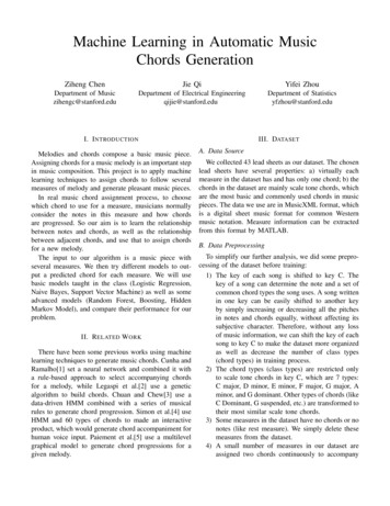
C. Support Vector Machine (SVM)E. BoostingSVM is one of the supervised learning algorithmswhich is to maximize the distance between trainingexample and classification hyperplane by finding (usehard-margin as an example):Boosting is a meta-algorithm to learn slowly to fitthe new model from the residual of the current model.Its parameters include the number of trees to split, theshrinkage parameter and the depth of the tree[6]. We alsoapplied this model in R.Specifically, we tune these parameters using cross validation to make sure the model has the best performance.As a result, the number of trees is 200, the shrinkageparameter is 0.2 and the depth is 4.minγ,w,b1 w 22s.t. y (i) (wT x(i) b) 1, i 1, ., m(5)By using kernel trick, SVM can efficiently performnon-linear classification or data with high-dimensionalfeatures. In this problem, we tried the following threekernels in R:1) Linear kernelK(xi , xj ) pXxip xjp(6)k 12) Polynomial kernelK(xi , xj ) 1 pX!dxip xjp(7)(xip xjp )2(8)k 13) Radial kernelK(xi , xj ) e γPpk 1D. Random ForestRandom forest is based on bagging which is a kindof decision tree with bootstrapping and can decreasevariance. For a classification problems with p features, p features are used in each split in order to decreasethe correlation of the trees[6]. We applied this modelusing R package.After applying the model, we can generate the importance plot for the features as the figure below. All thefeatures we are using have the similar importance level,which reinforces the conclusion from feature selection.F. Hidden Markov Model (HMM)Up till now, these five models above make predictionbased on the information of a single measure. We wantedto incorporate the relationship between measures. So, wealso tried HMM to make prediction based on a sequenceof measures.In HMM, the system is being modeled to be aMarkov process which has a series of observed statesx {x1 , x2 , ., xT } and a series of related unobserved(hidden) states z {z1 , z2 , ., zT } (T is the numberof the states). Suppose there are S types of observedstates and Z types of hidden states. An S S Transition Matrix denotes the transition probabilities betweenadjacent hidden states. And an S Z Emission Matrixdenotes the probabilities of each hidden state emit eachobserved state. Given an observed series of outputs, ifwe know the Transition Matrix and Emission Matrix,we can compute the most likely hidden series using theViterbi Algorithm[7].In our chord assignment problem, the first note of eachmeasure was considered as an observed state, and thechord of each measure was considered as a hidden state.Using our dataset, we computed the transition probabilityand emission probability and formed transition matrixand emission matrix. And then we computed the mostlikely chord progression using hmmviterbi function inStatistics and Machine Learning Toolbox in MATLAB.VI. R ESULTS & A NALYSISA. Cross ValidationFig. 2: Variable importanceWe started at comparing different machine learningmodels to indicate how they perform. We used hold-outcross validation and 30% of the data as the validationset. In addition, we also tried k -fold cross validation.The cross validation results are used to represent the testaccuracy and evaluate how our models perform.
B. Prediction on a Single MeasureThe cross validation accuracy for the five differentmodels we used is shown in TABLE III. (k 5, 10for k -fold)ModelLogistic RegressionNaive BayesSVM LinearSVM PolySVM RadialRandom .73%62.29%bias/low variance classifiers (e.g., Naive Bayes) couldhave a better performance. However, Naive Bayes alsoassumes that the features are conditionally independent.In reality, the four notes on the beat could influence eachother, so such strong assumption could limit the performance of Naive Bayes. Random forest and Boostingperform best in our case since they are both complexand have a reduction in model variance.C. Prediction on Sequential MeasuresThe following is the song m“silent night ” that isassigned chords by our HMM model.TABLE III: Accuracy for different modelsTo get an insight of the results above, we can havea look at the confusion matrix. Take SVM with radialkernel as an example: 45 0 1 6 1 6 2 0 5 0 0 0 0 0 0 0 0 0 0 0 0 5 2 0 13 1 3 1 (9) 2 1 1 1 4 0 0 1 0 0 1 3 3 1 0 0 0 0 0 0 3In the confusion matrix, the rows represent the prediction results, the columns represent the true labels and thediagonal values are the correct predictions. We can seethe data is highly imbalanced, i.e., most of the labels are1 or 4. In fact, for key C, the frequent chords are exactlyC major (1) and F major (4). This data distribution willcause our models to suffer.Now let’s visualize the accuracy results in the figurebelow.Fig. 4: Generated lead sheet based on HMM predictionsFig. 3: Visualization of accuracy for different modelsAs the figure shows, random forest and boosting arethe most solid models. Apart from the imbalanced data,logistic regression and SVM with linear kernel have badperformance, mainly because the relation is highly nonlinear and these models cannot fit this dataset while highThe result we get for HMM varies greatly for differentsongs. The overall accuracy of HMM is 48.44% but forsome pieces, it can achieve an accuracy over 70%. Thiscould be caused by the limited information provided bythe first note pitch observed. To add more pitches andregard a group of notes in the measure as an observation,the result can be improved but it will greatly complicatethe model with a much larger state space.The second reason is that, assigning chord is a moresubjective than objective process. Two composers maychoose different chord types for the same measure andboth of them can sound pleasant. There is no single normto decide if the chord is assigned correct or not.
VII. C ONCLUSION & F UTURE W ORKFrom the results above, we can conclude that Randomforest and Boosting perform best in prediction withsingle measure. HMM could also achieve a good resultif we include more information as our observation states.But the highest accuracy we can achieve is only about70%. This is caused by the subjectivity in our dataset.This can be improved by choosing data from onecomposer with one genre. However, it is typically hardto achieve. A better way is to design an experiment touse human judgements to evaluate the performance ofour model instead of only relying on the given labels.R EFERENCES[1] Cunha, U. S., & Ramalho, G. (1999). An intelligent hybrid modelfor chord prediction. Organised Sound, 4(02), 115-119.[2] Legaspi, R., Hashimoto, Y., Moriyama, K., Kurihara, S., &Numao, M. (2007, January). Music compositional intelligencewith an affective flavor. In Proceedings of the 12th internationalconference on Intelligent user interfaces (pp. 216-224). ACM.[3] Chuan, C. H., & Chew, E. (2007, June). A hybrid system forautomatic generation of style-specific accompaniment. In 4th IntlJoint Workshop on Computational Creativity.[4] Simon, I., Morris, D., & Basu, S. (2008, April). MySong:automatic accompaniment generation for vocal melodies. InProceedings of the SIGCHI Conference on Human Factors inComputing Systems (pp. 725-734). ACM.[5] Paiement, J. F., Eck, D., & Bengio, S. (2006). Probabilisticmelodic harmonization. In Advances in Artificial Intelligence(pp. 218-229). Springer Berlin Heidelberg.[6] James, G., Witten, D., Hastie, T., & Tibshirani, R. (2013). Anintroduction to statistical learning (p. 6). New York: springer.[7] Viterbi, A. J. (1967). Error bounds for convolutional codesand an asymptotically optimum decoding algorithm. InformationTheory, IEEE Transactions on, 13(2), 260-269.
Statistics and Machine Learning Toolbox in MATLAB. VI. RESULTS & ANALYSIS A. Cross Validation We started at comparing different machine learning models to indicate how they perform. We used hold-out cross validation and 30% of the data as the validation set. In addition, we also tried k-fold cross validation.