WIXLIB

Music Genre ClassificationMichael Haggblade1Yang HongKenny KaoIntroductionMusic classification is an interesting problem with many applications, from Drinkify (a program thatgenerates cocktails to match the music) to Pandora to dynamically generating images that complement the music. However, music genre classification has been a challenging task in the field of musicinformation retrieval (MIR). Music genres are hard to systematically and consistently describe dueto their inherent subjective nature.In this paper, we investigate various machine learning algorithms, including k-nearest neighbor (kNN), k-means, multi-class SVM, and neural networks to classify the following four genres: classical, jazz, metal, and pop. We relied purely on Mel Frequency Cepstral Coefficients (MFCC) tocharacterize our data as recommended by previous work in this field [5]. We then applied the machine learning algorithms using the MFCCs as our features.Lastly, we explored an interesting extension by mapping images to music genres. We matched thesong genres with clusters of images by using the Fourier-Mellin 2D transform to extract features andclustered the images with k-means.22.1Our ApproachData Retrieval ProcessMarsyas (Music Analysis, Retrieval, and Synthesis for Audio Signals) is an open source softwareframework for audio processing with specific emphasis on Music Information Retrieval Applications. Its website also provides access to a database, GTZAN Genre Collection, of 1000 audiotracks each 30 seconds long. There are 10 genres represented, each containing 100 tracks. All thetracks are 22050Hz Mono 16-bit audio files in .au format [2]. We have chosen four of the mostdistinct genres for our research: classical, jazz, metal, and pop because multiple previous work hasindicated that the success rate drops when the number of classifications is above 4 [4]. Thus, ourtotal data set was 400 songs, of which we used 70% for training and 30% for testing and measuringresults.We wrote a python script to read in the audio files of the 100 songs per genre and combine theminto a .csv file. We then read the .csv file into Matlab, and extract the MFCC features for eachsong. We further reduced this matrix representation of each song by taking the mean vector andcovariance matrix of the cepstral features and storing them as a cell matrix, effectively modelingthe frequency features of each song as a multi-variate Gaussian distribution. Lastly, we appliedboth supervised and unsupervised machine learning algorithms, using the reduced mean vector andcovariance matrix as the features for each song to train on.2.2Mel Frequency Cepstral Coefficients (MFCC)For audio processing, we needed to find a way to concisely represent song waveforms. Existingmusic processing literature pointed us to MFCCs as a way to represent time domain waveforms asjust a few frequency domain coefficients (See Figure 1).1

To compute the MFCC, we first read in the middle 50% of the mp3 waveform and take 20 ms framesat a parameterized interval. For each frame, we multiply by a hamming window to smooth the edges,and then take the Fourier Transform to get the frequency components. We then map the frequenciesto the mel scale, which models human perception of changes in pitch, which is approximately linearbelow 1kHz and logarithmic above 1kHz. This mapping groups the frequencies into 20 bins bycalculating triangle window coefficients based on the mel scale, multiplying that by the frequencies,and taking the log. We then take the Discrete Cosine Transform, which serves as an approximationof the Karhunen-Loeve Transform, to decorrelate the frequency components. Finally, we keep thefirst 15 of these 20 frequencies since higher frequencies are the details that make less of a differenceto human perception and contain less information about the song. Thus, we represent each raw songwaveform as a matrix of cepstral features, where each row is a vector of 15 cepstral frequencies ofone 20 ms frame for a parameterized number of frames per song.We further reduce this matrix representation of each song by taking the mean vector and covariancematrix of the cepstral features over each 20ms frame, and storing them as a cell matrix. Modeling the frequencies as a multi-variate Gaussian distribution again compressed the computationalrequirements of comparing songs with KL Divergence.Figure 1: MFCC Flow33.1TechniquesKullback-Lieber (KL) DivergenceThe fundamental calculation in our k-NN training is to figure out the distance between two songs.We compute this via the Kullback-Leibler divergence [3]. Consider p(x) and q(x) to be the twomultivariate Gaussian distributions with mean and covariance corresponding to those derived fromthe MFCC matrix for each song. Then, we have the following:However, since KL divergence is not symmetric but the distance should be symmetric, we have:3.2k-Nearest Neighbors (k-NN)The first machine learning technique we applied is the k-nearest neighbors (k-NN) because existingliterature has shown it is effective considering its ease of implementation. The class notes on knearest neighbors gave a succinct outline of the algorithm which served as our reference.3.3k-MeansFor unsupervised k-means clustering to work on our feature set, we wrote a custom implementationbecause we had to determine how to represent cluster centroids and how to update to better centroidseach iteration. To solve this, we chose to represent a centroid as if it were also a multi-variate Gaussian distribution of an arbitrary song (which may not actually exist in the data set), and initializedthe four centroids as four random songs whose distances (as determined by KL divergence) wereabove a certain empirically determined threshold. Once a group of songs is assigned to a centroid,the centroid is updated according to the mean of the mean vectors and covariance matrices of those2

songs, thus represented as a new song that is the average of the real songs assigned to it. Finally, asrandom initialization in the beginning and number of iterations are the two factors with notable influence on the cluster outcomes, we determined the iteration number empirically and repeatedly runk-means with different random initial centroids and pick the best, as determined by the calculatedtotal percent accuracy.3.4Multi-Class Support Vector Machine (DAG SVM)A directed acyclic graph of 2-class SVMs3.5SVM classifiers provide a reliable and fast way todifferentiate between data with only two classes.In order to generalize SVMs to data falling intomultiple classes (i.e. genres) we use a directedacyclic graph (DAG) of two-class SVMs trainedon each pair of classes in our data set (eg f14 (x)denotes the regular SVM trained on class 1 vsclass 4) [1]. We then evaluate a sequence of twoclass SVMs and use a process of elimination todetermine the output of our multi-class classifier.Neural NetworksWe tried neural networks because it has proved generally successful in many machine learningproblems. We first pre-process the input data by combining the mean vector and the top half of thecovariance matrix (since it is symmetric) into one feature vector. As a result, we get 15 (1 15) 152features for each song. We then process the output data by assigning each genre to an element in theset of the standard orthonormal basis in R4 for our four genres, as shown in the table below:GenreVectorClassical(1, 0, 0, 0)Jazz(0, 1, 0, 0)Metal(0, 0, 1, 1)Pop(0, 0, 0, 1)We then split the data randomly by a ratio of 70-15-15: 70% of the data was used for training ourneural network, 15% of the data was used for verification to ensure we dont over-fit, and 15% ofthe data for testing. After multiple test runs, we found that a feedforward model with 10 layers (seeFigure 2) for our neural network model gives the best classification results.Figure 2: Diagram of a Neural Network44.1ResultsMusic Genre ClassificationClassification accuracy varied between the different machine learning techniques and genres. TheSVM had a success rate of only 66% when identifying jazz , most frequently misidentifying itas classical or metal. The Neural Network did worst when identifying metal with a 76% successrate. Interestingly, the Neural Network only ever misidentified metal as jazz. k-Means did wellidentifying all genres but Jazz, which was confused with Classical 36% of the time. k-NN haddifficulty differentiating between Metal and Jazz in both directions. Of its 33% failures identifyingJazz, it misidentifies as Metal 90% of the time. Similarly, k-NN incorrectly predicted that Metal3

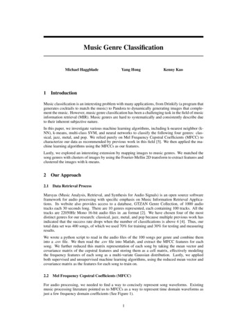
PredictedTable 3: k-Means ResultsActualClassical Jazz 88%61% 93%Pop0032890%PredictedPop1002997%Table 2: Neural Network 24Metal0013Pop100Accuracy88%100% 76%Table 4: k-NN ResultsActualClassical Jazz 7%67% 80%PredictedPredictedTable 1: DAG SVM ResultsActualClassical Jazz 7%67% 87%songs would be Jazz in 66% of all its failed Metal identifications. Overall we found that k-NNand k-means yielded similar accuracies of about 80%. A DAG SVM gave about 87% accuracy andneural networks gave 96% accuracy.4.2Music to Image MappingFigure 3: Image accompanying Lady Gaga’s Poker FaceAs an extension, we mapped images to song genres. We obtained 120 images, with 30 imagesof similar ”type” (i.e. nature images for classical music) per music genre. For extracting a setof features from the images, we used the Fourier-Mellin 2D transform (FMT), which is similar toextending MFCCs to 2D [6]. The main differences are that we binned the DTFT according to anon-uniform logarithmic grid and then transformed from cartesian to log-polar coordinates (keepingthe rest of the procedure more or less the same as MFCCs). This makes the Mellin 2D transforminvariant to rotation, scale, and illumination, which is important in image characterization.We then applied k-Means clustering to our feature matrices from FMT, using the Frobenius norm asour distance measure between images. Lastly, we matched each of the resulting clusters to a genre,such that given a song, we can map the song to a genre as well as to a random image in the associatedimage cluster. Our music to image mapper generated some fairly interesting results. For example,our music classification correctly identified Lady Gaga’s Poker Face song as Pop. When we thenmapped the pop genre to a random image from its associated image cluster, we received the imagein Figure 3, a very reasonable matching.4Pop00019100%Pop2102790%