Transcription
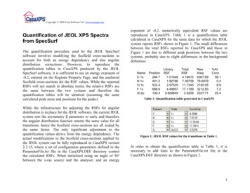
Copyright 2008 Casa Software Ltd. www.casaxps.comQuantification of JEOL XPS Spectrafrom SpecSurfThe quantification procedure used by the JEOL SpecSurfsoftware involves modifying the Scofield cross-sections toaccount for both an energy dependency and also angulardistribution corrections. However, to reproduce thequantification tables in CasaXPS produced by the JEOLSpecSurf software, it is sufficient to use an energy exponent of-0.2, entered on the Regions Property Page, and the unalteredScofield cross-sections for the RSF values. While the reportedRSFs will not match in absolute terms, the relative RSFs arethe same between the two systems and therefore thequantification tables will be identical (assuming the samecalculated peak areas and positions for the peaks).While the infrastructure for adjusting the RSFs for angulardistribution is in place for the JEOL software, the current JEOLsystem sets the asymmetry β parameter to unity and thereforethe angular distribution function returns the same value for alltransitions, hence the Scofield cross-sections are all scaled bythe same factor. The only significant adjustment to thequantification values derive from the energy dependency. Theactual modifications to the Scofield cross-sections applied bythe JEOL system can be fully reproduced in CasaXPS version2.3.15, where a set of configuration parameters defined in theParameterFile.txt file in the CasaXPS.DEF directory controlthe calculated RSFs. When initialised using an angle of 56ºbetween the x-ray source and the analyser, and an energyexponent of -0.2, numerically equivalent RSF values arereproduced in CasaXPS. Table 1 is a quantification tablecalculated in CasaXPS for the same data for which the JEOLsystem reports RSFs shown in Figure 1. The small differencesbetween the total RSFs reported by CasaXPS and those inFigure 1 are due to different peak positions between the twosystems, probably due to slight differences in the backgrounddefinition.NameC 1sN 1sO 1sF 1sSi 53212.832337.71%AtConc58.10.48.97.225.4Table 1: Quantification table generated in CasaXPSFigure 1: JEOL RSF values for the transitions in Table 1.In order to obtain the quantification table in Table 1, it isnecessary to add lines to the ParameterFile.txt file in theCasaXPS.DEF directory as shown in Figure 2.1
Copyright 2008 Casa Software Ltd. www.casaxps.comThe default CasaXPS library is populated with Scofield crosssections. These Scofield cross-sections are computed fromHartree-Slater wave-functions and therefore are appropriate foran XPS instrument designed with the, so called, magic anglebetween the x-ray source and the analyser axis. Given the anglebetween the x-ray source and the analyser, a correction can bemade to these magic angle RSFs appropriate for the giveninstrument. The configuration file in Figure 2 shows themethod for specifying the require angle for the JEOLinstrument, which is 56º. Each time one or more files areopened in CasaXPS for which the angle has yet to be set, adialog window prompts the user for the missing angle andoffers the configured angle as the default.Figure 2: ParameterFile.txt file in the CasaXPS.DEF directory used inversion 2.3.15 of CasaXPS.The JEOL element library includes the asymmetry parametersand therefore, should these be implemented in future releasesof the JEOL software the line in the ParameterFile.txt file “jeolangular distribution” would need to be changed to “correct forangular distribution”. With this adjustment, CasaXPS wouldextract RSFs from a Scofield library to include the full angulardistribution correction.Once a file is updated with an entry in the VAMAS filecomment of the form “SourceAnalyserAngle: 56.000000 d”,the source to analyser angle is defined for that file. Whencoupled with the configuration entry, “jeol angulardistribution”, the magic angle Scofield cross-sections from theelement library will be adjusted each time an RSF is extractedfrom the element library for use with a Region or Component.The column in Table 1 headed Total RSF is calculated fromthe RSF in the Region or Component multiplied by the energydependence defined by the value in the text-field on theRegions property page.The theory behind the use of angular distribution correction isdiscussed in detail elsewhere in the CasaXPS manual. Anoutline of the procedure will be given below.2
Copyright 2008 Casa Software Ltd. www.casaxps.comQuantification ExamplesThe follow examples illustrate how to quantify data from the JEOL JPS-9200 instruments at University of Wageningen, TheNetherlands.3
Copyright 2008 Casa Software Ltd. www.casaxps.comQuantification of a Survey Spectrumspectrum displaying element marks for oxygen, carbon andsilicon in preparation for creating regions using the CreateRegion button.Survey spectra are typically used to measure elementalconcentrations and therefore quantification regions are usuallythe tool of choice to measure the peak areas. A low resolutionacquisition mode enhances the signal-to-noise in a surveyspectrum, but broadens the peaks in the data making thesepeaks less appropriate for chemical state analysis by peakmodelling, hence the use of regions only. The first exampledescribes how to quantify a survey spectrum usingquantification regions.The Quantification Parameters dialog window is available fromthe Options menu on the CasaXPS main window or via the toptoolbar button. Quantification Regions are edited on theRegions property page on the Quantification Parameters dialogwindow, where the limits of integration, background type andRSF parameters are set. For successful quantification of asample using a survey spectrum, a set of Regions must becreated with the appropriate RSFs for the transitions identified.To ensure the correct RSF is extracted from the elementlibrary, the best means of creating regions for survey spectra isto use the Element Library dialog windowto create theregions. Buttons labelled Create Regions are on both theElement Table property page (Figure 3) and the Periodic Tableproperty page. These Create Regions buttons use the set ofelement marks currently defined on the survey spectrum toinitialise a set of regions on the data. Figure 4 shows a surveyFigure 3: Element Library Dialog Window4
Copyright 2008 Casa Software Ltd. www.casaxps.comOnce the element marks are defined for the data, simplypressing one of the Create Region buttons on the ElementLibrary dialog window will create a set of quantificationregions for the spectrum. If a peak can be identifiedcorresponding to the transitions with the largest RSF for eachelement, a region is created. If no peak can be detected, but it isdesired to include a region for a “missing peak”, then a furthermechanism to force the inclusion of a region is provided viathe Create When Line Selected tick box on the Element Tableproperty page. When ticked and the Region property page onthe Quantification Parameter dialog window is the top mostpage on the dialog window, selecting a transition from theElement Table causes a quantification region to be createdbased on the library entry just selected coupled with the currentdisplay window in the active tile. It is therefore advisable tozoom into the energy interval over which the new region mustcover before clicking on the Name field in the Element Table.A further consequence of creating regions using the CreateRegions button on the Element Library dialog window is thecreation of an annotation table offering a quantification reportwhich is displayed over the data as shown in Figure 5. Whilethe automatic creation of the quantification regions and reportis convenient, it is also advisable to check the limits for thequantification regions to ensure the backgrounds are definedappropriately for the data.Figure 4: Element markers defined using the Element Library dialogwindow in preparation for creating quantification regions.An easy way to investigate the region definitions is to press theReset buttonon the second toolbar and then sequentiallypress the Zoom Out button. The action of pressing theReset button is that of loading the limits for each region5
Copyright 2008 Casa Software Ltd. www.casaxps.comdefined on the spectrum in the active tile onto the current zoomlist. Each time the Zoom Out toolbar button is pressed, theregions, one-by-one, are displayed in the active tile. If theRegions property page is the top most property page on theQuantification Parameters dialog window, then the regionlimits can be adjusted using the left mouse-button to drag avertical cursor marking the start or end energies for the region.Once each region has been visited, the final press of the ZoomOut toolbar button will display the full spectrum.The Regions property page in Figure 6 corresponds to the datain Figure 5. Note how the RSFs in Figure 6 are adjusted usingthe configuration parameters in Figure 2 for the angulardistribution correction, while the energy dependency exponentdefined in Figure 2 appears on the Regions property page inFigure 6, but is not included in the RSFs reported on theRegions property page. Although the RSFs in Figure 6 differfrom the underlying Scofield cross-sections, the ratios of theseRSFs to the C 1s value are still in the relative proportions ofthe Scofield cross-sections and therefore simply using theScofield cross-sections with the energy dependency exponentof -0.2 is sufficient to obtain the SpecSurf quantification.Figure 5: Quantification regions created using the Create Regionsbutton on the Element Table property page.6
Copyright 2008 Casa Software Ltd. www.casaxps.comQuantification of Similar DataThe survey spectrum in Figure 5 is one of four spectra acquiredfrom different positions on a sample. The sequence ofexperiments appear in CasaXPS as shown in Figure 7, where inaddition to the survey spectra, high resolutions spectra arerecorded at each of the four sample positions.Figure 7: Right-hand-side of the Experiment Frame showing the set ofspectra in a VAMAS file.Figure 6: Regions property page showing the parameters used to createthe table over the spectrum in Figure 5.Given that the survey spectra are all similar in peak structure,elemental quantification for each of the four sample positionscan be obtained by propagating the regions define on thespectrum in Figure 5 to the other three survey spectra in thefile. To propagate regions from one spectrum to other spectra,display the spectrum for which the regions are already definedin the active display tile in the left-hand-side of the experimentframe and select the target VAMAS blocks in the right-handside, before right-clicking the mouse with the cursor over theactive tile displaying the quantified spectrum. A dialog windowappears as shown in Figure 8 in which the source VAMASblock is indicated and a list of target VAMAS blocks displays7
Copyright 2008 Casa Software Ltd. www.casaxps.comboth the block identifier string of the VAMAS blocks and thefilename in which the VAMAS blocks are located. Propagationis not limited to the file containing the source VAMAS block,but any open VAMAS files for which VAMAS blocks areselected can be targeted by the propagation operation.The actions taken on pressing the OK button on the dialogwindow in Figure 8 are determined by the tick-boxes in thePropagate section. The state of the Browser Operations inFigure 8 causes the regions from the survey spectrum measuredfrom sample position 2 in Figure 7 and defined by Figure 6 tobe transferred to the three other survey spectra.Figure 9: Report Spec Property Page.Generating Quantification ReportsFigure 8: Browser Operations dialog window.Differences between the compositions of the sample at thesefour positions can be examined by generating a quantification8
Copyright 2008 Casa Software Ltd. www.casaxps.comreport via the Report Spec property page on the QuantificationParameters dialog window. A tabulation of the quantificationvalues determined from the regions defined on the VAMASblocks selected in Figure 7 is generated by pressing the Regionbutton in the Standard Report section of the Report Specproperty page shown in Figure 9. The report shown in Figure10 can be saved to file via the File menu or transferred throughthe clipboard to a spreadsheet program using the Copy toolbarbutton (Ctrl C).adjusted on a sample by sample basis to ensure the appropriateC 1s peaks appear at the same binding energies. Locating apeak accurately for the purposes of energy calibration oftenrequired peak modeling of the data envelope. Once a peakenergy offset has been established, the same energy calibrationoffset must be applied to other data acquired under the sameexperimental conditions.The format for the quantification reports can be defined usingthe RegionQuantTable.txt file in the CasaXPS.DEF directory.The format for the Standard Report configuration files isdescribed elsewhere in the CasaXPS manual.Quantification of High Resolution SpectraHigh resolution spectra are typically acquired where chemicalstate information is required or elemental peaks overlap. Thelower pass energy used to acquire the spectra achieves betterenergy resolution for the peaks but at the cost of reducedintensity. The improved peak resolution transforms the broadpeaks of the survey mode into peaks for which peak positionsare significant in interpreting the data and therefore energycalibration is of greater importance to these high resolutiondata.The CasaXPS window shown in Figure 11 includes two C 1sspectra acquired from two different samples. The chargecompensation for these two experiments is clearly different andtherefore the spectra acquired from the two samples must beFigure 10: Standard Report generated by pressing the Region buttonon the Report Spec property page.9
Copyright 2008 Casa Software Ltd. www.casaxps.comFigure 11: VAMAS file written by SpecSurf including high resolution spectra from two samples.10
Copyright 2008 Casa Software Ltd. www.casaxps.comCreating a Peak ModelThe objective in creating a peak model for both the C 1sspectra shown in Figure 11 is to systematically establish theposition of the largest peak in each of the C 1s spectra as areference for calibrating the other high resolution data acquiredunder the same experimental conditions as the respective C 1sspectrum.combined string “C 1s” matches the name field in the elementlibrary, on pressing the Create button on the Regions propertypage a quantification region is created using the RSF derivedfrom the element library.Before synthetic peaks can be created, a quantification regionmust be defined on the C1s spectrum. The purpose of thequantification region is to specify the background type and thelimits over which the background approximation should apply.The Regions property page on the Quantification Parametersdialog window (Figure 6) is used to create the region requiredby the peak model. Creating a quantification region for the C1s spectrum is made simpler by virtue of the correct assignedto the spectrum of the element/transition fields in the VAMASfile. This is in contrast to the survey spectra, where it is notpossible to assign an element/transition owing to the fact thatall elements and transitions are present in the survey data.Both C 1s spectra in Figure 11 display regions defined with aTougaard background created via the Create button on theRegions property page. Background types are defined using theBG Type field on the Regions property page. The defaultbackground type is the most recently used background type andcan be altered by entering the character “L” for Linear, “S” forShirley or “T” for Tougaard before pressing the Enter key.Many other background types are available and are describeelsewhere in the CasaXPS manual, however for everyday usethese three as normally sufficient. Of the three most commonlyused background types, the Tougaard background is the leastused, however for the data in Figure 11 the background beginsto rise is such a way that both the Shirley and linearbackground fail to include the left-most C 1s peak.The data in the VAMAS file are organized in the right-handside of the experiment frame using the element/transition fieldsto arrange the data into columns, whereas the rows of VAMASblocks are defined by the experimental variable value, hencethe arrangement seen in Figure 11. Given that theelement/transition is correctly assigned, in the sense that theThe peaks in a peak model are created using the Componentsproperty page illustrated in Figure 12. The creation ofcomponent peaks is achieved by pressing the Create button onthe Component property page. Again, since theelement/transition fields defined in the VAMAS blockcontaining the C 1s spectrum match the correct entry in the11
Copyright 2008 Casa Software Ltd. www.casaxps.comelement library, the RSF derived from the element library isassigned to each component as it is created.Figure 12: Components Property PageThe components appear as columns on the Componentsproperty page, where the parameters are initialized usinginformation gathered from the C 1s data. The components aredefined in terms of a lineshape plus area, FWHM and positionparameters. Constraints are applied to the numerical parameterseither as intervals or by expressing the relationship betweentwo component parameters using the alphabetical labels abovethe columns on the Components property page. For example,the components defined on the C 1s spectrum corresponding tothe property page in Figure 12 are constrained to all have thesame FWHM. The fwhm Constr. field shown in Figure 12indicates that the parameter for column B and column C arecalculated from the FWHM value in column A using the stringA*1. Similarly, a known relationship between the areaparameter for two peaks can be applied with strings using thecolumn headers. For example, a doublet pair such as Si 2p1/2and Si 2p3/2 can be constrained in relative area using B*2, say,where the Si 2p1/2 component appears in column B, thecomponent for Si 2p3/2 appears in column A and the string B*2is entered into the Area Constr. field in column A. For positionconstraints, the separation of two peaks can be definedsimilarly using strings of the form A 0.25, say, in the Pos.Constr. field.Once a set of components are defined on a spectrum withappropriate constraints, the Fit Component button is pressedto optimize the fit to the data. Figure 13 shows the result offitting for the C 1s spectra in Figure 11. The constraint appliedto the FWHM provides a stabilizing influence on the peakmodel which permits the same model to apply to both C 1sspectra in Figure 11. By constructing a peak model suitable for12
Copyright 2008 Casa Software Ltd. www.casaxps.comboth sets of data, a consistent peak position can be establishedfor component C 1s 5, which in turn can then be used as thereference point for calibrating the energy scale for both sets ofspectra.energy for the C 1s peaks in Figure 13. These shifts in recordedbinding energy are due to different equilibrium charge statesfor the sample surfaces. It is assumed the same equilibriumcharge state influences the spectra from the same experimentacquired at different binding energies. VAMAS blocks with thesame position experimental variable will typically require thesame energy calibration therefore the calibration determinedfor the C 1s spectra must be applied to the other high resolutionspectra in the VAMAS blocks belonging to the same row inFigure 11.Figure 13: Optimized components representing chemically shifted C 1stransitions.Calibrating the Energy Scale for an ExperimentThe data in Figure 11 are two independent acquisitionconditions, which explain the different measured bindingFigure 14: Calibration property page.13
Copyright 2008 Casa Software Ltd. www.casaxps.comThe Calibration property page on the Spectrum Processingdialog windowpermits the specification of the measuredand true binding energies corresponding to a spectrum. Usingthese two energy values a shift is calculated, which can beapplied to a specific VAMAS block or, using the Apply toSelection button, to a set of VAMAS blocks. The procedure forcalibrating the energy scale for the two rows of data in Figure11 involves:1. Display the C 1s spectra in the active tile.2. Using the Calibration property page, enter the measuredvalue or the component C 1s 5 and the desired truevalue of 285.0 into the text-field labeled True.3. Select the VAMAS blocks for which the energycalibration is appropriate, i.e. those high resolutionspectra in the same row as the C 1s spectrum.4. Tick the tick boxes for Adjusting the region limits andcomponent parameters. This is required for spectrawhere regions and/or components are defined prior toenergy calibration.5. Press the Apply to Selection button on the Calibrationproperty page shown in Figure 14.The above five steps must be performed for each of the rowsshown in Figure 11. The calibration of the data is recorded inthe processing history for each VAMAS block and so can beviewed and modified on a spectrum-by-spectrum basis. Theconsequence of calibrating the two C 1s spectra using thecomponent C 1s 5 as the reference can be seen in Figure 15.These calibration shifts applied to the other spectra in the fileresult in relative peak positions shown in Figure 16.Figure 15: C 1s spectra after energy calibration.Assuming the calibration peak is correctly assigned for bothsamples and the sample equilibrium charge state for the Si 2pspectra is the same as the C 1s data, then a conclusion from theenergy calibration in Figure 16 is that the silicon chemical stateis different between the two samples.14
Copyright 2008 Casa Software Ltd. www.casaxps.comcontribution whilst using quantification regions for the N 1s, F1s, O 1s and Si 2p spectra. Two observations are worth noting:1. The high resolution spectra are all acquired using thesame pass energy and lens mode. Unless an instrumentis rigorously calibrated for intensity, quantification ofdata from different operating modes should be avoided.Transmission correction is a complex subject and isdealt with in detail elsewhere in the CasaXPS manual.Quantification using TAGs is a method for combiningquantification tables from different operating modes,which is again dealt with in detail elsewhere in theCasaXPS manual.Figure 16: The high resolution spectra from Figure 11 after calibrationusing the energy shifts performed for the C 1s data in Figure 15.Standard Report Quantification using HighResolution SpectraThe high resolution data in Figure 11 can be quantified againstone another by defining a set of components for the carbon2. The silicon doublet spectrum is assigned incorrectly aselement/transition of Si 2p3/2. When a region orcomponent is created using the Create button on therespective property pages, the wrong RSF for thedoublet pair will be extracted from the CasaXPSlibrary. Either the element/transition fields will need toadjusted prior to creating the region or the RSF updatedafter creation using #Si 2p entered in the name field ofthe region or the component.VariableC 1s1C 1s2C 1s3C 1s4C 1s5C sSi2p0.48.97.225.422.18.58.726.4Table 2: Atomic Concentration Table measured using components forthe C 1s and regions for all other spectra.15
Copyright 2008 Casa Software Ltd. www.casaxps.comThe quantification table in Table 2 is obtained from the data inFigure 15 and Figure 16 using the Region and Comps button inthe Standard Report section of the Report Spec property page(Figure 9). The atomic concentrations in Table 2 are computedusing both regions from the N 1s, O 1s, F 1s and Si 2p, whilethe intensity from the C 1s spectrum is measured using thecomponents rather than the region. Given that a region must bedefined on the C 1s spectrum, to avoid counting the carbonsignal twice, the RSF for the C 1s region must be assigned avalue of zero, while each of the components fitted to the C 1sdata are assigned the non-zero RSF for C 1s.Each of the buttons within the Standard Report may beconfigured using ASCII files located in the CasaXPS.DEFdirectory; specifically, the Regions and Comps button isconfigured using the RegionComponentQuantTable.txt file.Provided the Use Config File tick-box is ticked before pressingthe Regions and Comps button, the configuration filedetermines the format for the report. The report table can betransferred via the clipboard to a spreadsheet program bypressing the Copy button on the top toolbar (Ctrl C). Theclipboard selection dialog window resulting from the Copytoolbar button includes not only the data tabulated using theconfiguration file, but also a list of other tabulations for thequantification data. Additional formats are also generatedwithin the set of possible quantification tables by also tickingthe Use Profile Format tick-box. Table 2 derives from one ofthe profile format tables.16
Copyright 2008 Casa Software Ltd. www.casaxps.comTile DisplayFigure 17: Example of display format using Inset Tiles, Component colouring options and Peak Annotation.17
Copyright 2008 Casa Software Ltd. www.casaxps.comPresentation of data for reports and publication is an importantfeature to most researchers. The display of data in CasaXPS iscontrolled via the Tile Display Parameters dialog window,Page Tile Format dialog window and the Inset Tile mechanism.Once a display format has been prepared, such as the oneshown in Figure 17, the formatting information can be saved tofile and restored to the data at a later time using options on theFile menu (Figure 18) of CasaXPS.Figure 18: File Menu options for saving and loading tile display formatfiles.The Tile Display Parameter Dialog is available from theOptions menu and also the top toolbar. Display parametersaffecting fonts, colours for spectra and components, andselective display options such as labels on the axes are allfound on property pages on the Tile Display Parameter dialogwindow (Figure 19). The number of display tiles per page isFigure 19: Tile Display Parameter Dialog Windowcontrolled by the Page Tile Format dialog window(Figure20). Each property page on the dialog window represents apredefined format for the given number of tiles per page.Figure 16 illustrates the format for four tiles per page. Adetailed description of these display options can be found inThe Casa Cookbook and elsewhere in the CasaXPS help files.Figure 20: Page Tile Format Dialog Window18
system sets the asymmetry β parameter to unity and therefore the angular distribution function returns the same value for all transitions, hence the Scofield cross-sections are all scaled by the same factor. The only significant adjustment to the quantification values derive from the energy dependency. The