Transcription
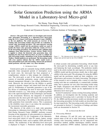
2012 IEEE Third International Conference on Smart Grid Communications (SmartGridComm), pp. 528-533, 5-8 November 2012Solar Generation Prediction using the ARMAModel in a Laboratory-level Micro-gridRui Huang, Tiana Huang, Rajit GadhSmart Grid Energy Research Center, Mechanical Engineering, University of California, Los Angeles, USANa LiControl and Dynamical Systems, California Institute of Technology, USAAbstract—The goal of this article is to investigate and researchsolar generation forecasting in a laboratory-level micro-grid,using the UCLA Smart Grid Energy Research Center (SMERC)as the test platform. The article presents an overview of theexisting solar forecasting models and provides an evaluation ofvarious solar forecasting providers. The auto-regressive movingaverage (ARMA) model and the persistence model are used topredict the future solar generation within the vicinity of UCLA.In the forecasting procedures, the historical solar radiation dataoriginates from SolarAnywhere. System Advisor Model (SAM)is applied to obtain the historical solar generation data, withinputting the data from SolarAnywhere. In order to validate thesolar forecasting models, simulations in the System IdentificationToolbox, Matlab platform are performed. The forecasting resultswith error analysis indicate that the ARMA model excels atshort and medium term solar forecasting, whereas the persistencemodel performs well only under very short duration.I. I NTRODUCTIONCurrent power grids are constantly facing reliable problemsespecially when unexpected periods of interruption occur.In recent years, the micro-grid has been proposed as acomplimentary solution to help mitigate the reliability issues. The micro-grid, as part of the smart grid realization,consists of renewable generation, energy storage units anddemand management through a low-voltage distribution network. Moreover, the micro-grid has the abilities to quicklyrespond to dynamic changes and island itself from the maingrid [1]. Proliferation of renewable generation is one of thekey drivers of establishing the need of micro-grid. Presently,renewable resources, e.g., solar energy, are employed globallydue to the rapid development of the technologies and benefitsto the environment. However, the integration of renewablegeneration into the micro-grid will require the assistant fromforecasting. Forecasting is the ability to determine periods ofstable generation from renewable sources. This is paramountto the reliability issues since it can reduce the uncertainty ofthe inconsistent renewable generation.The objective of the article is to study solar generationforecasting in a laboratory-level micro-grid. The UCLA SmartGrid Energy Research Center (SMERC) performs researchfocusing on the integration of solar generation in a laboratorylevel micro-grid [2], [3], [4]. Components of the laboratorylevel micro-grid consist of solar PV panels, battery storageunits and laboratory loads, such as laptops, LEDs and electricvehicles. The architecture of the laboratory-level micro-gridis displayed in Figure 1. Prediction models are developedFigure 1. The laboratory-level micro-grid with solar PV panels, batterystorage units and lab loads for the UCLA SMERCto obtain accurate solar generation forecasting, which benefitthe micro-grid by determining available power at any timeand balancing the loads accordingly. The prediction modelsused in the article include the auto-regressive moving average(ARMA) model and the persistence model, due to their applicability in the micro-grid. The advantages for using the ARMAmodel and the persistence model are their simplicity, costeffectiveness and accuracy for timely forecasting. The purposeof the research is not to compete with a variety of solar forecasting tools that are academically or commercially availabletoday, but to generate our own solar forecasting results usingthe simple, inexpensive and effective methods, based on theenvironment of UCLA, which can be implemented for thelaboratory-level micro-grid.Section II summarizes various existing forecasting methods.In addition, an investigation into the existing academic andcommercial forecasting tools is provided. In Section III andIV, the ARMA and the persistence models are introduced, andthe forecasting procedures for both models are described stepby-step respectively. The forecasting results with error analysisare presented in Section V. Conclusion of findings and futurework are documented in Section VI.II. L ITERATURE R EVIEWA. Forecasting MethodsBoth references [5] and [6] carry out surveys on thecurrent status of the art in solar forecasting. Essentially, theexisting solar forecasting methods can be categorized intopersistence method, satellite data/imagery method, numericweather prediction (NWP) method, statistical method and
hybrid method. A general overview of the solar forecastingmethods is presented in Table I.Table IS UMMARY OF THE FORECASTING METHODSMethodPersistenceSatellite Data/ImageryNWPStatisticalHybridDescriptionHigh correlationsbetween past and futureData analysis andimage processingPhysical modelMathematicalmodelCombination ofdifferent approachesTime HorizonVery short termExampleCAISOShort termUCSDLong termShort andmedium termAdjustableUCSDUCLACAISOThe simplest way to perform a solar forecasting is to usepersistence method. California Independent System Operator(CAISO) uses persistence method in its renewable energyforecasting and dispatching [7]. This method is highly effective in very short term prediction, i.e., 1 hour-ahead. Itis often used as a comparison to other advanced methods.References [8] and [9] describe the method based on satellitedata/imagery. Satellite data/imagery provides important atmospheric and meteorological information on cloudiness, cloudmotion vector, etc., for predicting the solar irradiance. Thismethod is evaluated to be the best method for 1 to 5 hourahead forecasting according to reference [5]. NWP methodmodels solar radiation in the air with consideration of thecloud layers in the forecasting process. It is deemed to bethe most successful method for long term solar forecasting,e.g., day-ahead, at present. Results from NWP method exhibithigher accuracy for longer time horizons as presented in references [10] and [11]. Statistical method develops mathematicalmodels which include auto-regressive with exogenous input(ARX), ARMA, auto-regressive integrated moving average(ARIMA) and artificial neural network (ANN). This methodis based on training the historical data spanning over a longtime period, e.g., one year, to tune the model coefficients.References [10], [12] and [11] use ARX, ARIMA and ANNto predict the solar generation respectively. They perform wellin the time horizons ranging from 1 hour up to 36 hours,which are short and medium term forecastings. In practice, asnumerous articles concluded, hybrid method is a combinationof different approaches that can be applied to obtain an optimalsolar prediction. For example, references [5] and [6] bothrecommend a combination of NWP method and a statisticalpost-processing tool as a promising option for solar prediction.B. Forecasting ToolsIn this section, we explore the existing academic solarforecasting tools and commercial solar forecasting providers.Most of the forecasting tools and providers apply the satellitedata/imagery and NWP methods. According to the investigation, Green Power Research offers solar forecasting serviceand solar resource assessment based on geostationary operational environmental satellite imagery, for utilities, independent system operators (ISO) and solar power producers[13].3Tier offers a solar predictor based on NWP method, withthe integration of cloud forecasting capability [14]. AWSTruepower (AWST) offers a solar forecasting system basedon NWP method, with statistical procedures for cloud patterntracking [15]. SolarAnywhere offers solar forecasting up to 7day-ahead based on satellite data such as cloud motion vectorfor short term forecasting, and NWP method for long termforecasting [16]. SolarCasters offers solar predictions for dayahead and hour-ahead, and delivers both irradiance forecasting and plant-specific generation forecasting using TRNSYSsimulation software based on NWP method, with proprietaryradiative transfer models to predict the irradiance reaching theground [17]. SOLARFOR offers solar power predictions for0-48 hour-ahead based on NWP method [18]. Atmosphericand Environmental Research (AER) Solar Forecast offers solarforecasting based on satellite data observations and NWPmethod, as well as with proprietary radiative transfer models[19]. Solar2000 offers solar irradiance forecasting at 1 to1, 000,000 nm throughout the solar system based on NWPmethod, with measuring sun rotation and infrared wavelength[20].III. F ORECASTING S ETUP FOR THE ARMA MODELThe ARMA model, also known as the Box–Jenkins model(1976), is one type of the time-series models in statisticalmethod. It can be used to solve the problems in the fields ofmathematics, finance and engineering industry that deal witha large amount of observed data from the past. The modeldescription and forecasting procedure for the ARMA modelare explained as below.A. Model DescriptionThe ARMA model is developed using Equation 1. It consistsof two parts, the auto-regressive (AR) part and the movingaverage (MA) part.pqXXS(t) αi S(t i) βj e(t j)(1)i 1j 1In Equation 1, S(t) is the forecasted solar generation at timet. In the AR part, p is the order of the AR process, and αi is theAR coefficient. In the MA part, q is the order of the MA errorterm, βj is the MA coefficient and e(t) is the white noise thatproduces random uncorrelated variables with zero mean andconstant variance [21]. Typically, this method requires a largeamount of historical data, e.g., one year, to obtain the ARMAmodel. That is to find the orders p, q and the coefficientsαi , βj . In addition, due to the geographical differences, eachlocation corresponds to its own unique model. Based on thegiven historical data, the construction of the model for eachlocation consists of two phases, identifying the orders p, qand determining the coefficients αi , βj . In particular, we limitp, q 10 to simplify the process. The algorithms to realizethe model are discussed in Step III-B3.B. Forecasting ProcedureThe five steps below are followed to complete the forecasting process.
Figure 2.Hourly GHI in 2010 for the UCLA SMERCFigure 3. Hourly solar generation simulated by SAM with 1 kW PV in 2010for the UCLA SMERC1) Obtain the historical solar radiation data: Since weaim to forecast the solar generation for the laboratory-levelmicro-grid, the traces of historical solar generation data areused as the input of the ARMA model. In the first step, wecollect hourly solar radiation data from SolarAnywhere, a webbased service that offers hourly global horizontal irradiance(GHI), direct normal irradiance (DNI) and diffuse horizontalirradiance (DHI) for locations within the U.S.A. that datesfrom 1998 to 2011 [16]. The data we collect covers the entireyear from Jan. 1st, 2010 to Dec. 31st, 2010 for the vicinityof UCLA, California (latitude 34.065, longitude -118.445).The Figure 2 shows the hourly GHI in 2010 for the UCLASMERC, which is the most essential solar radiation data forgenerating solar energy.2) Simulate the historical solar generation data: We useSystem Advisor Model (SAM) to produce the hourly solargeneration data from Jan. 1st, 2010 to Dec. 31st, 2010, withinputting the hourly solar radiation data from SolarAnywhere.As a performance-based model in the renewable energy industry, SAM can promptly assist the decision making processin various aspects of solar power generation [22]. To bemore specific, it has functions of modeling PV system andsimulating the solar production. Our design of the PV systemin SAM is composed of a desired array (size of 1 kW dc),a module (SAM/Sandia Modules/SunPower SPR-210-BLK[2007(E)]) and a grid-connected PV inverter (capacity of 4 kWac). The solar generation data simulated by SAM is shown inFigure 3. It is estimated that the total solar generation in 2010for the UCLA SMERC is 3.324 MW and the peak is 1.7491kW with the average of 0.3795 kW.3) Realize the ARMA model: The mathematical methodsof finding the orders and coefficients of the ARMA modelare introduced in reference [23]. The order identification isproposed by Daniel and Chen (1991), and coefficients determination is calculated by applying the Yule-Walker relations forαi and the Newton-Raphson algorithms for βj . In the article,the two-phase realization of the ARMA model is implementedin the System Identification Toolbox, Matlab platform [24]. Byinputting the data resulted from SAM into Matlab, the SystemIdentification Toolbox is capable of constructing mathematicalmodels, i.e. finding the orders and coefficients in Equation 1.As a result, the realized ARMA model is able to deliver time-series output for forecasting in the next step.4) Predict the future values: The future values can bepredicted using the realized ARMA model. For example,Equation 2 is applied to predict the h hour-ahead forecasting(h 1, 2, 3.hours).S(t h) pXαi S(t i) i 1qXβj e(t j)(2)j 1where S(t h) is the forecasted solar generation at time t h.5) Analyze the errors: In order to measure the accuracy ofthe predictions, the errors between the forecasted values andactual data are analyzed here. In the forecasting procedure,we train the hourly solar generation data for 2010 to obtainthe ARMA model, and use the model to forecast the hourlysolar generation values for 2011, for the UCLA SMERC. Inthe article, Mean Absolute Error (MAE) and Mean SquaredError (MSE), defined in Equation 3 and 4, are used as theerrors to validate the prediction method.nM AE 1X A(t) F (t) n t 1vu nX1uM SE t (A(t) F (t))2n t 1(3)(4)where n is the length of the time horizon, i.e., n 744 ifwe choose January for the time horizon, and A(t) and F (t)denote the actual data and the forecasted value at time t.In the forecasting procedure, the historical data are for 2010from Step III-B2, the forecasted values are for 2011 from StepIII-B4 and the actual data are for 2011 from SAM. The dataentered into SAM are the solar radiation data for 2011 fromSolarAnywhere.IV. F ORECASTING S ETUP FOR THE PERSISTENCE MODELA. Persistence ModelAs a comparative study, the persistence model is developedusing Equation 5 to predict the h hour-ahead forecasting (h
1, 2, 3.hours).S(t h) S(t)(5)where S(t h) is the forecasted solar generation at time t h.B. Forecasting ProcedureSimilarly, the forecasting procedure for the persistencemodel includes obtaining the historical solar radiation datafrom SolarAnywhere, simulating the historical solar generation data by SAM, predicting the future values by applyingEquation 5 and analyzing the errors. Differently, the historicaldata and the actual data are the same, both for 2011 fromSAM. The data entered into SAM are the solar radiation datafor 2011 from SolarAnywhere.Figure 4. 1 hour-ahead solar generation forecasting and actual data on Jan.1st, 2011 for the UCLA SMERCV. F ORECASTING R ESULTSA. The realized ARMA modelWe conduct the Matlab simulations to obtain the ARMAmodel. Table II presents the values of the orders and coefficients for the ARMA model for the UCLA SMERC.Table IIT HE REALIZED ARMA MODELpq23αiα1 1.597α2 0.6882βjβ1 0.2072β2 0.1768β3 0.0513B. The forecasted values and actual dataFigure 4 shows the curves of the forecasted solar generationand actual data for 1 hour-ahead on Jan. 1st, 2011 for thelaboratory-level micro-grid. Figure 5 shows the curves of theforecasted solar generation and actual data for 1 hour-aheadon Jul. 1st, 2011. There are at least three points that are ofinterest. On Jan. 1st, for the very short term forecasting, i.e., 1hour-ahead, the curve produced by the ARMA modelresembles the actual data from 6:00 AM to 11:00 AM butvaries considerably at a later time. In particular, there isa small fluctuation around 4:00 AM. However, such timeperiods cannot obtain much sunlight. Therefore, there isa need to improve the model by taking actual weatherdata into account in the future. On the other hand, the curve produced by the persistencemodel has a tiny shift along the time horizon compared tothe actual data. Nonetheless, this model is still accurate. On Jul. 1st, the ARMA model matches more closelyto the actual data than that on Jan. 1st. The ARMAmodel performs better in the prediction during the monthsthat have more sunlight. Similar errors are found around4:00 AM, which emphasize the importance of improvingthe ARMA model by considering actual weather data.Similarly, the persistence model performs well in the 1hour-ahead forecasting on Jul. 1st.Figure 6 and Figure 7 show the curves of the forecastedsolar generation and actual data for 3 hour-ahead on Jan.Figure 5. 1 hour-ahead solar generation forecasting and actual data on Jul.1st, 2011 for the UCLA SMERC1st and Jul. 1st, 2011 for the laboratory-level micro-gridrespectively. There are at least three points that are of interest. Both on these two days, the ARMA model presents betterpredictions than the persistence model for short termforecasting, i.e., 3 hour-ahead, which illustrates that thepersistence model is only accurate for very short termforecasting. For the predictions based on the ARMA model, it isevident that the results for 1 hour-ahead are better than3 hour-ahead. The prediction accuracy decreases as thehour-ahead increases. Similar trends can be found for the persistence model.The prediction accuracy decreases considerably as thehour-ahead increases.C. The Error AnalysisAs mentioned in Step III-B5, we use MAE and MSEto measure the accuracy. Figure 8 shows the distributionsof the MAE for each month during 2011 for 1 hour-aheadforecasting, for the ARMA model and the persistence modelrespectively. There are at least three points that are of interest. For each month of the year, the MAE of the ARMAmodel is smaller than the persistence model, whichtranslates into the conclusion that the ARMA model is
Figure 6. 3 hour-ahead solar generation forecasting and actual data on Jan.1st, 2011 for the UCLA SMERCFigure 7. 3 hour-ahead solar generation forecasting and actual data on Jul.1st, 2011 for the UCLA SMERC more reliable for 1 hour-ahead forecasting. Take Januaryas example, the ARMA model shows an improvement ofas much as 17.62% compared to the persistence model.The maximum MAE of the ARMA model is 0.1013 kWin March while the minimum MAE is 0.073 kW in July,with the average MAE of 0.0894 kW.The maximum MAE of the persistence method is 0.1322kW in April while the minimum MAE is 0.1033 kW inJanuary, with the average MAE of 0.1213 kW.Figure 9. The MSE of the ARMA model and the persistence model for 1hour-ahead forecasting for each month of 2011 for the UCLA SMERCFigure 9 shows the distributions of the MSE for each monthduring 2011 for 1 hour-ahead forecasting, for the ARMAmodel and the persistence model respectively. There are atleast three points that are of interest. Similar trends can be found in this comparison. TheMSE of the ARMA model is smaller than the persistencemodel, for each month of the year for 1 hour-aheadforecasting. Take January as example, the ARMA modelshows an improvement of as much as 44.38% comparedto the persistence model. The maximum MSE of the ARMA model is 0.028 kW inMarch while the minimum MAE is 0.0121 kW in July,with the average MAE of 0.0206 kW. The maximum MAE of the persistence model is 0.0502kW in September while the minimum MAE is 0.0356kW in January, with the average MAE of 0.042 kW.Figure 10 shows the variations of the MAE and the MSEfor different hour-ahead forecasting, in July, 2011. The hourahead ranges from 1 to 5. There are at least three points thatare of interest. As results illustrated, as the forecasting hour-ahead increases, the MAE and the MSE for each model increaseaccordingly. However, they increase by different degreesfor different models. Generally speaking, the errors of theARMA model are smaller than the persistence model. The errors in the ARMA model varies steadily. Whenthe hour-ahead is larger than 4, the MAE and the MSEalmost remain constant. The results further demonstratethat the ARMA model is suitable for short and mediumterm forecasting. The errors in the persistence model increase considerablyas the hour-ahead increases. The results further demonstrate that the persistence model is only suitable for veryshort term forecasting.VI. C ONCLUSIONSFigure 8. The MAE of the ARMA model and the persistence model for 1hour-ahead forecasting for each month of 2011 for the UCLA SMERCSolar generation can be gradually integrated into the powergrid starting at the micro-grid level, as the prominent powergeneration technology for the UCLA SMERC. Due to theunpredictability and variability of the current solar generation,
Figure 10. The MAE and MSE of the ARMA model and the persistencemodel in July, 2011 for different hour-ahead forecasting for the UCLASMERCthe wide adoption of solar generation forecasting is stillunderway.According to the reviews carried out in the article, based onthe assessment of solar forecasting methods, statistical methodperforms well for solar generation prediction especially forshort and medium term. Currently, academic and commercialforecasting models have their unique identities, and performwell depending on whether it is for short term or long termforecasting. We suggest that a combination of solar forecastingmodels should be used to solve the reliability issues associatedwith the integration of solar generation into the micro-grid.As discussed in the article, statistical method typically usestime-series models such as the ARMA model to obtain desirable forecasting results. We extract information from currentforecasting algorithms and produce our own forecasting procedure for the ARMA model. The procedure includes obtainingthe historical solar radiation data from SolarAnywhere, simulating the historical solar generation data by SAM, realizingthe ARMA model, predicting the future values and analyzingthe errors. In the meanwhile, we use the persistence modelas a comparison. The error analysis reveals that the ARMAmodel is preferred for short and medium term prediction on amicro-grid level. Moreover, results indicate that the persistencemodel performs well in very short term prediction.The next step is to produce a hybrid energy system thatincludes solar PV panels and battery storage units, in orderto realize the isolated operation for some periods of time.Continuous research is needed to establish hybrid method toimprove the prediction of its solar generation output.ACKNOWLEDGEMENTThis work is supported by Smart Grid Energy ResearchCenter (SMERC), UCLA, U.S.A. and Korean Institute ofEnergy Research (KIER), Korea.R EFERENCES[1] Agarwal, Y.; Weng, T.; Gupta, R.K.; , “Understanding the role ofbuildings in a smart microgrid,” Design, Automation & Test in EuropeConference & Exhibition (DATE), 2011, vol., no., pp.1-6, 14-18 Mar.2011.[2] “UCLA Smart Grid Energy Research Center (SMERC).” Smart Grid Energy Research Center. Web. 03 May 2012. http://smartgrid.ucla.edu/ .[3] S. Mal, A. Chattopadhyay, A. Yang, R. Gadh, “Electric vehicle smartcharging and vehicle-to-grid operation,” International Journal of Parallel,Emergent and Distributed Systems, vol. 27, no. 3. March 2012.[4] R. Gadh, presented at "Computational Needs for the Next GenerationElectric Grid workshop", Organized by Department of Energy, Hostedby Bob Thomas (Cornell University), Joe Ito (Sandia National Labs)and Gil Bindelwald (Department of Energy) April 18-20, 2011.[5] J. Kleissl, “Current Status of the Art in Solar Forecasting,” CaliforniaRenewable Energy Forecasting, Resource Data and Mapping FinalReport, Appendix A, 2010.[6] D. Heinemann, E. Lorenz and M. Girodo, “Forecasting of Solar Radiation,” Energy Meteorology Group, Germany, 2005.[7] Jian M.; Makarov, Y.V.; Loutan, C.; Zhijun X.; , “Impact of wind and solar generation on the California ISO’s intra-hour balancing needs,”Powerand Energy Society General Meeting, 2011 IEEE , vol., no., pp.1-6, 2429 Jul. 2011.[8] Bayer, H.G., Costanzo, C., Heinemann, D. and Reise, C., “Short RangeForecast of PV Energy Production Using Satellite Image Analysis,” Proc.12th European Photovoltaic Solar Energy Conference, 11-15 Apr., 1994,Amsterdam, 1781-1721.[9] A. Hammer, D. Heinemann, E. Lorenz and B. Lï¿œckehe, “Short-termforecasting of solar radiation: a statistical approach using satellite data,”Solar Energy, Volume 67, Issues 1–3, Jul. 1999.[10] P. Bacher, H. Madsen and H. A. Nielsen, “Online short-term solar powerforecasting,” Solar Energy, Volume 83, Issue 10, Oct. 2009.[11] Y. Huang, J. Lu, C. Liu, X. Xu, W. Wang and X. Zhou, “Comparativestudy of power forecasting methods for PV stations,” Power SystemTechnology (POWERCON), 2010 International Conference on , vol.,no., pp.1-6, 24-28 Oct. 2010.[12] Perdomo, R.; Banguero, E.; Gordillo, G.; , "Statistical modeling forglobal solar radiation forecasting in Bogotï¿œ," Photovoltaic SpecialistsConference (PVSC), 2010 35th IEEE , vol., no., pp.002374-002379,20-25 Jun. 2010.[13] ”Green Power Labs Solar Vision People.” Green Power Labs. Web. 19Apr. 2012. http://www.greenpowerlabs.com/buildings.html .[14] casting.3Tier,Inc.Web.17Apr.2012. http://www.3tier.com/en/package detail/powersight-solarforecasting/ .[15] “AWS Truepower: Solar Solutions: Forecasting and cienceDeliversPerformance.Web.17Apr.2012. sting-gridintegration/ .[16] erResearch.Web.17Apr.2012. https://www.solaranywhere.com/Public/Overview.aspx .[17] “Solar Demand Forecaster.” Technology Scouting. Lux Research.Web. 17 Apr. 2012. solar-demand-forecaster.html .[18] tor.”ENFOR.Web.17Apr.2012. http://www.enfor.dk/solar power prediction solarfor.php .[19] vironmentalResearch2002.Web.17Apr.2012. and-solance .[20] W.K. Tobiska, Status of the SOLAR2000 solar irradiance model, Physicsand Chemistry of the Earth, Part C: Solar, Terrestrial & PlanetaryScience, Volume 25, Issues 5–6, 2000.[21] Rajagopalan, S.; Santoso, S.; , “Wind power forecasting and erroranalysis using the autoregressive moving average modeling,” Power &Energy Society General Meeting, 2009. PES ‘09. IEEE , vol., no., pp.16, 26-30 July 2009.[22] boratory. Alliance for Sustainable Energy. Web. 2 May 2012. https://sam.nrel.gov/content/welcome-sam .[23] J. L. Torres, A. Garcia, M. De Blas and A. De. Francisco, “Forecastof hourly average wind speed with ARMA models in Navarre (Spain),”Solar Energy, Volume 79, Issue 1, pp. 65-77, Jul. 2005.[24] orks,Inc.Web.2May2012. 4wup.html .
2) Simulate the historical solar generation data: We use System Advisor Model (SAM) to produce the hourly solar generation data from Jan. 1st, 2010 to Dec. 31st, 2010, with inputting the hourly solar radiation data from SolarAnywhere. As a performance-based model in the renewable energy in-dustry, SAM can promptly assist the decision making process