Transcription
Exploring a Data Acquisition Device with LabviewA USB data acquisition device (Labjack U3-HV) is controlled via software (Labview) to sourcecurrent ( 0-10 mA) or voltage ( 0-3.5 V) and simultaneously measure current ( 0 -20 mA) orvoltage ( 0 – 7/10 V). A Labview code is available which can used (with appropriate inputs) toperform current vs. voltage I(V) and voltage vs. current V(I) sweeps on devices like diodes, LEDs etc.Other Labview codes available for the U3 should be explored. The students are free to create newmeasurement combinations using this. The aim of the exercise is to explore the functionality of the U3and understand its limitations.If interested students are encouraged to test the U3 with any other experiment available in the laboutside of lab hours.The experiment will closely be based on the attached paper. Some technical details will varydepending on the equipment available in the lab. The user manual of U3 is available online and also asa pdf file in the lab. Students are encouraged to visit the ‘Labjack website’ and read the manual to learnmore about the capabilities of the U3. Explore and come up with new ideas.Reference:P. Lecalir, M. Wofsey, J. Kuykendall and D. Whitcomb,“A low-cost system for introducing students to circuits and electrical propertiesbama.ua.edu/ pleclair/bamalab.pdfScroll down to see more
A low-cost system for introducing students to circuits and electrical propertiesP. LeClair,1, 2, Mike Wofsey,1 J. Kuykendall,1 and D. Whitcomb121Department of Physics and Astronomy, University of Alabama, Tuscaloosa, Al 35487Materials for Information Technology Center, University of Alabama, Tuscaloosa, Al 35487(Dated: August 1, 2007)The authors have developed a simple and inexpensive hands-on computerized tutorial aimed atintroducing beginning students to basic circuits and electrical properties. The system is capableof a wide variety of electrical measurements, including V (I) and I(V ) characteristics, voltage stepfunction response (e.g., charging and discharging capacitors), and time-dependent behavior using alow-frequency oscilloscope. The hardware is based on an inexpensive USB-data acquisition device.Freely-available custom software developed by the authors provides numerous experiment modules,and is designed to be highly extensible. The project can be implemented for 200 per seat, andhas recently been successfully utilized in an introductory general physics course at the University ofAlabama.I.INTRODUCTION AND MOTIVATIONElectronic devices have become ubiquitous in modernsociety. No matter how complex these devices, the electrical properties of their component materials and thebasic principles behind them remain the same. It is becoming increasingly crucial that students have a detailed,hands-on understanding of the basic principles of electriccircuits and the electronic properties of materials. Moreimportantly, the proper training of the next generationof scientists and engineers compels us, as instructors, tointroduce these concepts in a manner commensurate withwhat they will encounter in advanced laboratory coursesand research settings. This represents a significant challenge in terms of overall cost and flexibility to addresschanging needs. In this article, we present an examplesystem we believe meets these criteria at a minimum ofcost, the details of which we make freely available.1Within many disciplines, students are exposed to thebasic concepts of electronic devices and electrical properties of materials. However, providing students with amodern, hands-on approach to basic circuits and electrical property measurements resembling what they wouldfind in a research laboratory is often lacking. We believethis is due in no small part to the depth and breadthof knowledge required and the significant cost involvedin equipping a teaching laboratory with modern dataacquisition-based software and hardware. Not only isthis a major gap in students’ education, it is a seriousimpediment in many cases to their introduction to laboratory or industrial research. Far too often, teachinglabs seem hopelessly out of date for those of us workingdaily in related fields. Prior to this project, this was often the case for the authors, but cost alone prohibited acommercial solution to the problem. Our goal with thepresent system is to give students at least a glimpse ofhow electrical property measurements are performed ina modern research lab, at the minimum of cost.Many physics courses do currently employ a computerized hands-on approach to electronics and electronicproperties. Unfortunately, the cost can be prohibitive.Comparable systems to what we present here can coststhousands of dollars per seat. Further, proprietary commercial systems are rarely sufficiently open to extendor repair as instructional needs change – hardware isproprietary, software is closed-source, and electronic devices change rapidly. Finally, many commercial systemsare not sufficiently transparent for students to grasp theinner-workings of the underlying software and hardware– in the end, closed systems are in danger of being ‘blackboxes’ to the students, hiding many of the fundamentalaspects of electrical property measurement. The presentproject aims to provide a completely open and low-costsolution for students to perform experiments similarly tohow they are actually performed in research laboratories,and alleviate one barrier for promising students to beginresearch.In the hopes of addressing some of the issues outlinedabove, the authors have developed a simple and inexpensive hands-on computerized tutorial aimed at introducing students to basic circuits and electrical properties ofmaterials.1 Keeping hardware cost at a minimum, andfreely distributing software2 will allow, we hope, rapiduptake of the system by others. The project providesa complete hands-on system for modern data-aquisitionbased electrical transport measurements, for 200/seat.The software to run the data acquisition hardware, laboratory procedures, complete hardware schematics, assembly instructions – everything needed to build the hardware and install the software – is freely available online.The hardware itself is based on the LabJack U3 dataacquisition device3 ( 90 with educational discount), augmented only by a few passive components and a singleop-amp.4The software allows control over sourcing and measuring current and voltage, time-dependent behavior of RCcircuits, and a simple oscilloscope. I(V ), V (I), and V (t)curves can be measured and saved to simple ASCII filesfor post-analysis. The hardware is designed to be as inexpensive as possible, transparent, and easily assembled;the software, easily installed and rapidly parsed. Currently, the prototype system is complete, and has beenclassroom tested (20 units for 48 students) in Spring 2007
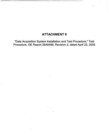
2in an introductory physics course.5In the spirit of keeping the system as simple as transparent as possible, as well as working within the hardwarelimitations inherent with our desire for minimal cost, weinitially created a list of working assumptions to guidethe effort. First, for an introductory laboratory class,we accept an accuracy of 5 10 % for teaching fundamental concepts. Second, components can be pre-selectedto avoid hardware and software limitations – componentsavailable to the students will not fall outside the measurable range. Third, the system must be portable, simple, and easily reproducible by colleagues without accessto technical support. Fourth, minimal cost and maximal simplicity override minor performance and accuracygains. Finally, the system must be as far as possible‘student-proof’ – so long as no external hardware is interfaced, the system must not be capable of destroyingitself!II.HARDWARELabJack U3 : The heart of the system is the LabJack U3 USB-based data acquisition and control device.3The U3 provides 16 software-configurable “flexible I/O”(FIO) terminals, which can be configured as digital input,digital output, and analog input, along with two timers,two counters, and four additional digital I/O connections.When configured as analog inputs, the FIOs provide 12bit resolution (0 2.4V single-ended, 2.4 V differential).Analog input reads typically take 0.6 4.0 msec. One dedicated 8-bit analog output (DAC0, 0 5 V) is available,with a second analog output (DAC1) available dependingon the software configuration. The U3 is USB driven andpowered, requiring no external supply connection. Theprimary advantages of the U3 from our point of view areextremely low cost6 ( 90, with educational discount; volume discounts available), flexibility, and an fairly opendriver interface. The U3 has several limitations whichmust be taken into consideration, however, which are relatively minor and easily worked around.One primary limitation of the LabJack U3 is that theanalog inputs are pseudo-bipolar – essentially, one canonly measure positive voltages. The 12-bit FIOs yieldonly 1 mV voltage resolution, limiting accuracy on voltage and current measurements. The FIOs also have arather low input impedance (20 kΩ), making meter loading a potential problem. The refresh rate (20 msec) andoutput frequency cutoff (3 dB at 16 Hz), to an extent restrict time-dependent measurements. Output voltagesare essentially limited to 3.6 V, and the fact that the U3is USB-powered severely limits overall current draw.Given these limitations, we employed a number of‘workarounds.’ In particular, the low refresh rate, lowinput impedance, and output frequency cutoff requireforethought in designing experiments, particularly wherecircuit time constants play a role. The simplest and mosteffective is carefully choosing the components for eachLabJackFIO 110kstudent box10kVin FIO 0Vin -FIO 3Iin FIO 2150Iin -DAC 1Vout GNDVout -FIG. 1: Schematics of the voltage input, voltage output, andcurrent input connections between the LabJack U3 and thelaboratory system. A 2:1 voltage divider increases the voltage input range of the LabJack, current measurements areperformed with a resistive shunt. Voltage is sourced directlyfrom the DAC.laboratory ahead of time, such that the students will notimmediately be aware of many limitations. When limitations are discovered, they can be used as an importantpedagogical tool for further instruction. We have foundthat students readily understand and accept hardwarelimitations, so long they can be explained.Other limitations are also not so serious on further reflection. The lack of true bipolar I/O requires manuallyreversing polarity and performing ‘positive’ and ‘negative’ measurements, which in some cases can provide aninstructional advantage. For example, measuring the forward I(V ) characteristic for a diode requires the studentto carefully observe polarity, rather than being able torely on simply changing the software parameters. Theinput voltage limitation is circumvented by the simpleaddition of a 2:1 voltage divider on voltage measuringinputs (see below), giving us a measurement range sufficient for most experiments.The first four FIOs are configured (in software) as differential analog inputs, which are used for current andvoltage measurements. The first analog output (DAC0)is used to drive a simple voltage-current converter forcurrent sourcing, and the second analog output (DAC1)provides voltage sourcing. Figure 1 shows the interfacingbetween the U3 and the I/O connections on the studentboxes.Measuring Voltage: Input voltage is measured between the FIO1 and FIO0 terminals (Fig. 1). This givesa rather limited input voltage range (0 3.6 V), and wetherefore connected the voltage input terminals “ Vin ”on the student box through a simple 2:1 voltage dividerto extend the measurement range.Measuring Current: Naturally the U3 measuresonly voltages, necessitating the need for a current to voltage converter. A simple resistive shunt is sufficient for
3this purpose, and current measurements are performedwith a shunt (150 Ω) between FIO3 and FIO2 analog inputs. So far as the students are concerned, this acts likea classic ammeter - it must be in series with the load.Nominally, this gives us a maximum measurable currentof 24 mA (due to the maximum FIO input voltage), anda minimum resolvable current change of 6 µA (due tothe FIO resolution). The output current of the studentboxes is limited to 10 mA, and the output voltage to 5 V, thus for judicious choice of loads, the 0 24 mA input current limit does not present a serious obstacle. Asmentioned above, we design laboratory procedures withlimitation in mind, and limit the selection of loads thestudents may use to work within the hardware limitations.Naturally, due to the rather large value of the shuntresistor, its non-negligible voltage drop must be takeninto account when doing, e.g. I(V ) characteristics. Wetake this as an opportunity to introduce the students toa true four-point measurement (see Fig. 5) and workingaround non-ideal meters and sources. By recognizing thehardware limitations and making them explicit, the students quickly learn to work within them and understandproper four-point measurements.Sourcing Voltage:The voltage output simply usesthe built-in analog output DAC1 referenced to ground(the first output, DAC0, is used for current output, seebelow). This limits the voltage range to 3.6 V, whichagain is adequate with careful component choice.Sourcing Current:: Sourcing current representedthe most difficult challenge within the constraints decidedupon. The U3, unfortunately, is not capable on its ownof driving sufficient currents, necessitating an additionalpower supply. The primary factor above all others isminimum cost, which eliminates a great many far moreelegant solutions. Portability was another prime issuein addition to cost and simplicity. Ideally, the systemshould not be tethered to a wall outlet, which precludesthe use of separate ac supplies to drive active elements.For this reason, the programmable current output isa very simple battery-powered voltage-to-current converter, driven by batteries, as shown in Fig. 2. Thevoltage-current converter essentially consists of onegeneral-purpose op-amp4 , and one programming resistor.The op-amp itself is supplied with two 9 V batteries. Weadded a DPST switch to open-circuit the batteries whennot in use, and battery test points on the outside of theproject box. Anecdotally, we did not replace a singlebattery in the 20 units over the course of a semester.The desired current level is programmed with theDAC0 output (0 3.6 V when using both analog outputs)on the U3, referenced to ground. The single programming resistor governs the ratio between input voltageand output current. In our case, Rprog 310 Ω yields3.2 mA/V in, for a maximum of about 10 mA output.This circuit allows only unipolar output, but as the LabJack itself is only pseudobipolar this is not an additionallimitation. (DAC0) --9V-IoutR(GND)battery test 9V- 9V-DPST 9V-9Vbattery test9VFIG. 2: Voltage-current converter circuit. The resistor Rselects the ratio between the input voltage and the outputcurrent. For portability, the op-amp is powered from 2-9 teryswitchbattery testFIG. 3: A finished student laboratory box.Finished Product: Figure 3 shows a completed system, housed in a 8x6x3 in project box.7 The total estimated cost per completed box was 160. We addedtransparent plexiglass covers for the boxes (not includedin cost estimate), in order to make the simplicity of theunderlying hardware as transparent as possible to thestudents. The U3 is (upper center) is held in placewith Velcro8 to allow for rapid replacement. More curious students can easily recognize the voltage dividerand current-measuring shunt resistor. Standard female’banana’ plugs9 are used for current and voltage input/output, while two female mini-banana plugs serve asbattery test points.10 The USB control cable and batteryswitch are also visible in the Fig. 3.
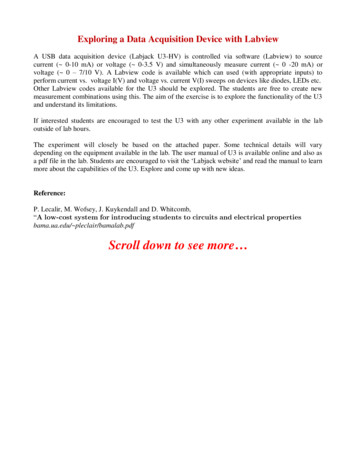
4III.SOFTWAREThe software was developed entirely by one of the authors (P.L.), using the LabWindows/CVI developmentpackage11 from National Instruments. All of the software for this project, excepting the LabJack driver andits interface, has been made freely available online1 underthe GNU General Public License.2 An emphasis has beenmade on simplicity of the user interface, and consistencyacross the modules as much as possible. For example, allmeasurement modules present identical parameter inputfields and graphing capabilities as far as possible, andadditional help is available through ‘tooltips’ at any timeby right-clicking on elements within windows. A simpleASCII configuration file or a GUI interface within thesoftware (“Settings” menu) allows field-tuning of hardware and software behavior by instructors (e.g., calibration factors, altering I/O settings). Most students appeared to find the software intuitive, with few questionsregarding usage. A usability study is underway to finetune the user interface, as is a comparative study withmore traditional approaches to the same laboratory procedures.The simplicity and modularity is reflected in the underlying code as well – the infrastructure allows new ormodified experimental modules to be coded and implemented in a minimum amount of time. Thus, as newideas develop they can be quickly realized. Extensivefeedback was solicited from students at all levels, faculty,and a software usability expert. In order to facilitateuptake of the system, a “demo mode” is automaticallyentered when no hardware is present. Potential userscan download the software, and explore the functionalityof the system free of cost. All software functionality ispresent to ‘test-drive’ the system, with actual measurements replaced by randomly-generated numbers.Multimeter : Different tutorial modules can be selected from the “main” applicaiton window, Fig. 4. Thefirst software module the students typically encounter isa ’multimeter’ panel, Fig. 4, chosen from the ‘dc circuits’menu. From this panel, the student can source currentor voltage, and simultaneously measure current or voltage, in any combination. Currents from 0 10 mA canbe sourced, and measured from 0 20 mA, while voltagescan be sourced from 0 3.5 V, and measured from 0 7 V.The multimeter panel is not meant to mimic the behavior of a hand-held multimeter precisely. Rather, itsgoal is to familiarize students with the basic practicesof sourcing and measuring currents and voltages. Whenthe multimeter module is selected from the “dc circuits”menu (Fig. 4), the source and measurement regions of themodule are blank until the user selects a source and measurement function. The two text areas at the bottom ofthe window give various instructions, which change as theuser interacts with the module. Initially, they prompt theuser to select a source and measurement function. Oncefunctionality has been chosen, the uppermost text arearelates to the chosen source (e.g., reminding the user thatFIG. 4: Left: A screenshot of the main application window.Right: A screenshot of the software, showing the ‘multimeter’panel. Current or voltage can be sourced or measured in anycombination, both source and measurement are updated inreal time. Active text areas at the bottom of the panel givethe user instructions for the selected source and measurement.the current source also has a switch), the lowermost tothe chosen measurement. In the case shown in Fig. 4,the user selected to source voltage, and measure current.Selecting voltage sourcing activates a dial, on/off button, indicator LED, and numerical readout (middle left).The user can either dial in the current or type a numberin the text box, and turn the source on or off with the labeled buttons. The ‘LED’ turns green when the source isactive, red when it is off. The current can be changed inreal-time (all sourcing and measuring is real-time, with 50 msec update time).Selecting current measurement activates a needlegauge, on/off button, indicator LED, and numerical readout (middle right). The on/off button starts and stopsthe readout, the status of which is also indicated by an‘LED.’ Both the numerical readout and needle gauge readthe current in real-time while active. Though strictlyspeaking only unipolar measurements are performed, thereadout is bipolar to help the student troubleshoot incorrect wiring (polarity reversal). Further, this panel allowsa quick ‘field calibration’ – e.g., by connecting the currentinput to the current output and electing to source andmeasure current. Similar behavior occurs when the user,e.g., sources voltage and measures current - the contentsof the window reflect the chosen source and measurement.Usually this panel is used for the very first dc circuitsexperiment, which simply has the students attempt tosource and measure current and voltage for three typesof components: resistors, diodes, and capacitors. Thisshort activity gives the students an introduction to keyelectrical components and basic wiring concepts as wellas an overview of the software they will utilize in laterlab sessions. Subsequently, the multimeter panel can beused to measure the equivalent resistance for series andparallel resistors, and directly verify that the current andvoltage, respectively, are the same for both resistors.Current vs. Voltage: The next level of complexity for the students is to perform current vs. voltagesweeps, I(V ), or voltage vs. current sweeps, V (I). Both
5Vin VVin -deviceunder testIin IIin Vout Vout -FIG. 5: Left: A screenshot of the software, showing a measurement of a 1350 Ω resistor using the current vs. voltagemodule. The maximum on the voltage axis does not correspond to the maximum sweep voltage, due to the finite resistance of the ‘ammeter.’ Right: Schematic of a four-terminalI(V ) measurement.FIG. 6: A module for observing voltage step responses. Applying stepped voltages (i.e., either suddenly turning a voltage on or off) allows real-time observation of charging and discharging behavior. Two successive measurements are shownon screen, one measuring the response of a series RC circuit,and one measuring the stepped output alone for comparison.sweeps are supported, and the software functionality isessentially identical. Both types of sweeps are providedfor two reasons: first, for non-linear components (e.g.,diodes) the characteristics appear different to studentsat first sight, and secondly, a true four-terminal measurement is qualitatively different in each case. We limitour discussion to the I(V ) functionality below.The I(V ) function is selected from the “dc circuits”menu on the main window (Fig. 4 ). A screenshot of thispanel is shown in Fig. 5. The “Control” region of thewindow (upper right) asks the user to specify the startand end voltages, and how many steps to take in between.The output is unipolar, and limited from 0 3.5 V asdiscussed above (the user will be coerced if values outsidethis range are specified). Sweeps can run “up” or “down”as desired.Once the desired values are chosen, clicking the blue“Start I(V)” button performs the measurement and updates the graph in real time. The ’LED’ in the upperright corner when the measurement is active. At anytime, the red “Halt” button can be pressed to immediately stop the measurement. After taking data, the twored crosshairs can be used to select a region of data, andthe ”zoom” button will rescale the plot to show only thatregion. “Restore” will auto-scale the plot to its originalstate. Data will remain on the plot (and in memory) untilthe “Clear” button is pressed. The small white crosshairis a plot read-out, and when dragged to a data point, the“Data display” in the lower right will indicate the current, voltage, and resistance (R VI ) at that data point.A text field in the lower left gives interactive status andinstructions, and, as in any panel, ‘tooltips’ are availableby right-clicking on objects within the panel.Measuring I(V ) characteristics quickly introduces thestudents to proper four-terminal measurements and theeffects of, e.g., finite wire and ammeter resistances. Inorder to perform a four-terminal measurement (Fig. 5)the student must connect the current measurement inseries with the load. Further, they must simultaneouslymeasure the actual voltage drop on the device under test,as a non-negligible voltage drop occurs across the 150 Ωshunt resistor in our ‘ammeter.’In any of the measurement panels (excepting the multimeter panel), any data currently on screen can be savedthrough the “File” menu. If multiple curves are takenwithout clearing the plot, all data currently on-screen issaved to the data file, not just the most recent data. Thedata itself is saved in a tab-delimited ASCII file, with aone-line text header for column labels, readily importedby e.g., Excel or OriginLab.In one example, students performed V (I) measurements for series and parallel resistor combinations, andperformed linear regression to find the effective resistance. Once simple resistor circuits have been mastered,students can be introduced to non-linear elements (suchas diodes). In particular, light-emitting diodes are anexcellent. Not only is non-linear behavior observed (andthus I(V ) and V (I) on first sight appear to be different), students can clearly see the device light up onlyfor a single voltage polarity. This also allows a brief introduction to semiconductor physics and non-linear regression. For example, comparing the threshold voltagefor light-emitting diodes of various colors to the outputwavelength (as measured with a diffraction grating), students were able to estimate Planck’s constant to within 10 %.12Step Response: The next level of complexity is mastering RC circuits and time-dependent phenomena. Figure 6 shows a module which allows characterization ofstep function responses. In one case, the student observes the response of a circuit to a downward voltagestep (from V to 0), in the other case, the response to anupward step is observed (from 0 to V ). This lets students monitor in real-time the charging and dischargingof a parallel RC circuit, for example.Measuring the discharge curve of an RC circuit, forexample, a user-selected constant voltage is applied fora specified wait time, and subsequently (at t 0 on theplot) the voltage is reduced to zero. This functionality isselected by choosing “initially” from the “Apply Voltage”
6FIG. 7: A module for learning the time-dependent behaviorof circuits. Students can apply a low-frequency waveform toa circuit (sine, square, triangle, or sawtooth), and observe theamplitude and phase behavior of the response. The drivingsinusoid and the response are measured simultaneously.drop-down menu. The actual voltage on the resistor orcapacitor can be monitored during this time, and the RCtime constant directly observed. Again, data can be easily exported for subsequent analysis, a good introductionto exponential and logarithmic behavior.The charging curve can be just as easily measured byselecting “After Delay” from the pull-down menu. In thiscase, the measurement proceeds for the specified timewith zero voltage, and at t 0 the specified voltage isapplied. This allows one to observe the correspondingcharging curve for an RC circuit, which is shown in Fig.6. Also shown is the step response itself, measured bysimply connecting voltage output to input. Given the20 kΩ input impedance of the LabJack FIOs, and thetime resolution of 10 msec, components giving a fairlylarge time constant ( 0.1 sec) should be selected.Oscilloscope: The last module completed at the moment mimics the behavior of an oscilloscope and functiongenerator. A variety of waveforms can be applied andplotted in real time, and the response of a circuit elementplotted at the same time. The waveforms are generatedin software, and limited by the refresh rate of the U3DAC and its output filters. A dc offset voltage is necessary to keep the output voltage at or above ground at alltimes, due to the pseudobipolar nature of the LabJackU3. This offset is automatically included without userintervention. Square, triangle, sawtooth, and sinusoidalwaveforms are currently supported and generated in software. In principle, arbitrarily complex waveforms can beadded in software as needed. Figure 7 shows the resultof applying a sinusoidal voltage to a resistive circuit, andFig. 8 to a parallel RC circuit. This allows direct observation of the phase-shifted response of a capacitor in anRC circuit, and an introduction to the frequency-domaindescription of ac circuits. In more advanced classes, onecan use, e.g., triangular or square waveforms to illustrateintegrating and differentiating RC circuits, or the effectsof ‘stray capacitance.’Peak to peak amplitude can be specified, up to 4 V, anda ‘Response Gain’ can be used to magnify the on-screenFIG. 8: Left: Measurement of the voltage on a 2200 µF capacitor in parallel with a 200 Ω resistor driven with a sinusoid.Right: Current-voltage characteristics for red, green, and yellow LEDs. Students compared the threshold voltage withmeasured output wavelengths to estimate Planck’s constant.signal for easier comparison (only ‘raw’ data is saved).Triggering is done in software after a specified number ofcycles – the default is to trigger every 3 cycles, but thisvalue is user configurable in the ‘Settings’ menu. Outputfrequency is limited primarily by the output filters on theLabJack DAC outputs (3 dB at 16 Hz), in practice 5 Hzprovides reasonable waveforms. Once again, by carefulchoice of components, this rather low frequency limitation need not be a problem. Induced voltages due totime-varying magnetic fields, and RLC resonant behavior are rather inaccessible given the available frequencyrange, however.Example measurements: Figure 8 shows two additional measurements performed with the present system.In the first case, the initial response to a sinusoidal excitation on a 2200 µF capacitor in para
Exploring a Data Acquisition Device with Labview A USB data acquisition device (Labjack U3-HV) is controlled via software (Labview) to source current ( 0-10 mA) or voltage ( 0-3.5 V) and simultaneously measure current ( 0 -20 mA) or . sive hands-on computerized tutorial aimed at introduc-ing students to basic circuits and electrical .