Transcription
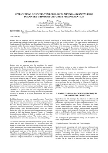
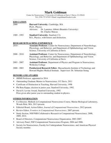
CHAPTERTemporal Data Miningfor Neuroscience15Wu-chun Feng, Yong Cao, Debprakash Patnaik, Naren RamakrishnanToday, multielectrode arrays (MEAs) capture neuronal spike streams in real time, thus providingdynamic perspectives into brain function. Mining such spike streams from these MEAs is criticaltoward understanding the firing patterns of neurons and gaining insight into the underlying cellularactivity. However, the acquisition rate of neuronal data places a tremendous computational burden onthe subsequent temporal data mining of these spike streams. Thus, computational neuroscience seeksinnovative approaches toward tackling this problem and eventually solving it efficiently and in realtime.In this chapter, we present a solution that uses graphics processing units (GPUs) to mine spike traindatasets. Specifically, our solution delivers a novel mapping of a “finite state machine for data mining”onto the GPU while simultaneously addressing a wide range of neuronal input characteristics. Thissolution ultimately transforms the task of temporal data mining of spike trains from a batch-orientedprocess towards a real-time one.15.1 INTRODUCTIONBrain-computer interfaces have made massive strides in recent years [1]. Scientists are now able toanalyze neuronal activity in living organisms, understand the intent implicit in these signals and,more importantly, use this information as control directives to operate external devices. Technologiesfor modeling and recording neuronal activity include functional magnetic resonance imaging (fMRI),electroencephalography (EEG), and multielectrode arrays (MEAs).In this chapter, we focus on event streams gathered through MEA chips for studying neuronal function. As shown in Figure 15.1, an MEA records spiking action potentials from an ensemble of neurons,and after various preprocessing steps, these neurons yield a spike train dataset that provides a real-timedynamic perspective into brain function. Key problems of interest include identifying sequences offiring neurons, determining their characteristic delays, and reconstructing the functional connectivityof neuronal circuits. Addressing these problems can provide critical insights into the cellular activityrecorded in the neuronal tissue.In only a few minutes of cortical recording, a 64-channel MEA can easily capture millions of neuronal spikes. In practice, such MEA experiments run for days or even months [8] and can result inGPU Computing Gemsc 2011 NVIDIA Corporation and Wen-mei W. Hwu. Published by Elsevier Inc. All rights reserved. 211
212CHAPTER 15 Temporal Data Mining for Neuroscience605040302010020.65 20.70 20.75 20.80 20.85 20.90 20.95 21.00Time (in sec)Frequent episodesGPGPU504030201002.138 2.140 2.142 2.1442.146 2.148 2.150Time (in sec)Microelectrode array 103Action potentials from real neuron cellsFIGURE 15.1Spike trains recorded from a multielectrode array (MEA) are mined by a GPU to yield frequent episodes, whichcan be summarized to reconstruct the underlying neuronal circuitry.trillions to quadrillions of neuronal spikes. From these neuronal spike streams, we seek to identify (ormine for) frequent episodes of repetitive patterns that are associated with higher-order brain function.The mining algorithms of these patterns are usually based on finite state machines [3, 5] and can handletemporal constraints [6]. The temporal constraints add significant complexity to the state machine algorithms as they must now keep track of what part of an episode has been seen, which event is expectednext, and when episodes interleave. Then, they must make a decision of which events to be used in theformation of an episode.15.2 CORE METHODOLOGYWe model a spike train dataset as an event stream, where each symbol/event type corresponds to aspecific neuron (or clump of neurons). In addition, the dataset encodes the occurrence times of theseevents.
15.2 Core Methodology213Temporal data mining of event streams aims to discover interesting patterns that occur frequentlyin the event stream, subject to certain timing constraints. More formally, each pattern (i.e., episode)is an ordered tuple of event types with temporal constraints. For example, the episode shown below1 after event A and at most t1describes a pattern where event B must occur at least tlowhigh after event A22and event C must occur at least tlow after event B and at most thigh after event B. 1 1 22(tlow ,thigh ] (tlow ,thigh ]A B CThe preceding is a size-three episode because it contains three events.Episodes are mined by a generate-and-test approach; that is, we generate numerous candidateepisodes that are counted to ascertain their frequencies. This process happens levelwise: search forone-node episodes (single symbols) first, followed by two-node episodes, and so on. At each level,size-N candidates are generated from size-(N-1) frequent episodes, and their frequencies (i.e., counts)are determined by making a pass over the event sequence. Only those candidate episodes whose countis greater than a user-defined threshold are retained. The most computationally expensive step in eachlevel is the counting of all candidate episodes for that level. At the initial levels, there are a large numberof candidate episodes to be counted in parallel; the later levels only have increasingly fewer candidateepisodes.The frequency of an episode is a measure that is open to multiple interpretations. Note that episodescan have “junk” symbols interspersed; for example, an occurrence of event A followed by B followedby C might have symbol D interspersed, whereas a different occurrence of the same episode might havesymbol F interspersed. Example ways to define frequency include counting all occurrences, countingonly nonoverlapped occurrences, and so on. We utilize the nonoverlapped count, which is defined as themaximum number of nonoverlapped instances of the given episode. This measure has the advantageousproperty of antimonotonicity; that is, the frequency of a subepisode cannot be less than the frequencyof the given episode. Antimonotonicty allows us to use levelwise pruning algorithms in our search forfrequent episodes.Our approach is based on a state machine algorithm with interevent constraints [6]. Algorithm 1shows our serial counting procedure for a single episode α. The algorithm maintains a data structures, which is a list of lists. Each list s[k] in s corresponds to an event type E(k) α and stores the times(k 1) (k 1)of occurrences of those events with event type E(k) that satisfy the interevent constraint (tlow , thigh ]with at least one entry tj s[k 1]. This requirement is relaxed for s[0], thus every time an event E(0)is seen in the data, its occurrence time is pushed into s[0].When an event of type E(k) , 2 k N at time t is seen, we look for an entry tj s[k 1] such(k 1) (k 1)that t tj (tlow , thigh ]. Therefore, if we are able to add the event to the list s[k], it implies thatthere exists at least one previous event with event type E(k 1) in the data stream for the currentevent that satisfies the interevent constraint between E(k 1) and E(k) . After we apply this argumentrecursively, if we can add an event with event type E( α ) to its corresponding list in s, then thereexists a sequence of events corresponding to each event type in α satisfying the respective intereventconstraints. Such an event marks the end of an occurrence, after which the count for α is incremented and the data structure s is reinitialized. Figure 15.2 illustrates the data structure s for counting(5,10](10,15]A B C.
214CHAPTER 15 Temporal Data Mining for NeuroscienceAlgorithm 1: Serial Episode Mining.(1) (1)(tlow ,thigh ]Input: Candidate N-node episode α E(1) . . . E(N) and event sequence S {(Ei , ti ) i 1 . . . n}.Output: Count of nonoverlapped occurrences of α satisfying interevent constraints1: count 0; s [[], . . . , []] //List of α lists2: for all (E, t) S do3:for i α down to 1 do4:E(i) ith event type of α5:if E E(i) then6:iprev i 17:if i 1 then8:k s[iprev ] 9:while k 0 do10:tprev s[iprev , k](iprev )(iprev )11:if tlow t tprev thigh then12:if i α 1 then13:count ; s [[], . . . , []]; break Line: 1.214:else15:s[i] s[i] t16:break Line: 1.217:k k 118:else19:s[i] s[i] t20: RETURN countEvents: AABBATimes: 125810 13 15 18 E 15.2(5,10](10,15]An illustration of the data structure s for counting A B C.15.3 GPU PARALLELIZATION: ALGORITHMS AND IMPLEMENTATIONSTo parallelize the aforementioned sequential counting approach on a GPU, we segment the overallcomputation into independent units that can be mapped onto GPU cores and executed in parallel to
15.3 GPU Parallelization: Algorithms and Implementations215fully utilize GPU resources. Different computation-to-core mapping schemes can result in differentlevels of parallelism, which are suitable for different inputs for the episode counting algorithm. Next,we present two computation-to-core mapping strategies, which are suitable for different scenarios withdifferent sizes of input episodes. The first strategy, one thread per occurrence of an episode, is used formining a very few episodes. The second strategy is used for counting many episodes.15.3.1 Strategy 1: One Thread per OccurrenceProblem ContextThis mapping strategy handles the case when we have a few input episodes to count. In the limit,mining one episode with one thread severely underutilizes the GPU. Thus, we seek an approach toincrease the level of parallelism. The original sequential version of the mining algorithm uses a statemachine approach with a substantial amount of data dependencies. Hence, it is difficult to increasethe degree of parallelism by optimizing this algorithm directly. Instead, we transform the algorithmby discarding the state-machine approach and decomposing the problem into two subproblems thatcan be easily parallelized using known computing primitives. The mining of an episode entails counting the frequency of nonoverlapped neuronal patterns of event symbols. It represents the size of thelargest set of nonoverlapped occurrences. Based on this definition, we design a more data-parallelsolution.Basic IdeaIn our new approach, we find a superset of the nonoverlapped occurrences that could potentially beoverlapping. Each occurrence of an episode has a start time and an end time. If each episode occurrencein this superset is viewed as a task/job with fixed start and end times, then the problem of findingthe largest set of nonoverlapped occurrences transforms itself into a job-scheduling problem, wherethe goal is to maximize the number of jobs or tasks while avoiding conflicts. A greedy O(n) algorithmsolves this problem optimally where n is the number of jobs. The original problem now decomposesinto two subproblems:1. Find a superset of nonoverlapped occurrences of an episode2. Find the size of the largest set of nonoverlapped occurrences from the set of occurrencesThe first subproblem can be solved with a high degree of parallelism as will be shown later inthis chapter. We design a solution where one GPU thread can mine one occurrence of an episode. Topreprocess the data, however, we perform an important compaction step between the searches of thenext query event in the episode. This entailed us to investigate both a lock-based compaction methodusing atomic operations in CUDA as well as a lock-free approach with the CUDPP library. However,the performance of both compaction methods was unsatisfactory. Thus, in order to further improveperformance, we adopted a counterintuitive approach that divided the counting process into three parts.First, each thread looks up the event sequence for suitable next events, but instead of recording theevents found, it merely counts and writes the count to global memory. Second, an exclusive scan isperformed on the recorded counts. This gives the offset into the global memory where each thread canwrite its “next events” list. The actual writing is done as the third step. Although each thread looks upthe event sequence twice (first to count and second to write), we show that we nevertheless achievebetter performance.
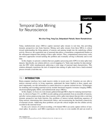
216CHAPTER 15 Temporal Data Mining for NeuroscienceThe second subproblem is the same as the task or interval scheduling problem where tasks havefixed times. A fast greedy algorithm is well known to solve the problem optimally.Algorithmic ImprovementsWe first preprocess the entire event stream, noting the positions of events of each event type. Then, fora given episode, beginning with the list of occurrences of the start event type in the episode, we findoccurrences satisfying the temporal constraints in parallel. Finally, we collect and remove overlappedoccurrences in one pass. The greedy algorithm for removing overlaps requires the occurrences to besorted by end time, and the algorithm proceeds as shown in Algorithm 2. Here, for every set of consecutive occurrences, if the start time is after the end time of the last selected occurrence, then we selectthis occurrence; otherwise, we skip it and go to the next occurrence.Next, we explore different approaches of solving the first subproblem, as presented earlier. The aimhere is to find a superset of nonoverlapped occurrences in parallel. The basic idea is to start with allevents of the first event-type in parallel for a given episode and find occurrences of the episode startingat each of these events. There can be several different ways in which this can be done. We shall presenttwo approaches that showed the most performance improvement. We shall use the episode A(5 10](5 10] B C as our running example and explain each of the counting strategies using this example. Thisexample episode specifies event occurrences where an event A is to be followed by an event B within5–10 ms and event B is to be followed by an event C within 5–10 ms delay. Note again that the delayshave both a lower and an upper bound.Parallel Local TrackingIn the preprocessing step, we have noted the locations of each of the event-types in the data. In thecounting step, we launch as many threads as there are events in the event stream of the start eventtype (of the episode). In our running example these are all events of type A. Each thread searches theevent stream starting at one of these events of type A and looks for an event of type B that satisfies theinter event time constraint (5 10]; that is, 5 tBj tAi 10 where i, j are the indices of the events oftype A and B. One thread can find multiple B’s for the same A. These are recorded in a preallocated arrayassigned to each thread. Once all the events of type B (with an A before them) have been collected bythe threads (in parallel), we need to compact these newfound events into a contiguous array/list. Thisis necessary because in the next kernel launch we will find all the events of type C that satisfy theinterevent constraints with this set of B’s. This is illustrated in Figure 15.3.Algorithm 2: Obtaining the Largest Set of Nonoverlapped Occurrences.Input: List C of occurrences with start and end times (si , ei ) sorted by end time, ei .Output: Size of the largest set of nonoverlapped occurrences.Initialize count 0preve 0for all (si , ei ) C doif preve si thenpreve ei ; count count 1return count
15.3 GPU Parallelization: Algorithms and Implementations217Iteration CTime (in sec)Iteration #2EventsAThread-1Thread-3Thread-4Thread-2BCTime (in sec)FIGURE 15.3Illustration of the parallel local tracking algorithm (i.e., Algorithm 3), showing two iterations for the episodeA B C with implicit interevent constraints. Note that each thread can find multiple next events.Furthermore, a thread stops scanning the event sequence when event times go past the upper bound of theinterevent constraint.Algorithm 3: Kernel for Parallel Local Tracking.Input: Iteration number i, Episode α, α[i]: ith event-type in α, Index list Iα[i] , Data sequence S.Output: Iα[i 1] : Indices of events of type α[i 1].for all threads with distinct identifiers tid do(i) (i)Scan S starting at event Iα[i] [tid] for event-type α[i 1] satisfying inter-event constraint (tlow , thigh ].Record all such events of type α[i 1].Compact all found events into the list Iα[i 1] . Iα[i 1]Algorithm 3 presents the work done in each kernel launch. In order to obtain the complete set ofoccurrences of an episode, we need to launch the kernel N 1 times where N is the size of an episode.The list of qualifying events found in the ith iteration is passed as input to the next iteration. Someamount of bookkeeping is also done to keep track of the start and end times of an occurrence. After thisphase of parallel local tracking is completed, the nonoverlapped count is obtained using Algorithm 2.The compaction step in Algorithm 3 presents a challenge because it requires concurrent updates into aglobal array.Implementation NotesLock-Based CompactionNVIDIA graphics cards with CUDA compute capability 1.3 support atomic operations on shared andglobal memory. Here, we use atomic operations to perform compaction of the output array into theglobal memory. After the counting step, each thread has a list of next events. Subsequently, each threadadds the size of its next events list to the block-level counter using an atomic add operation and, in
218CHAPTER 15 Temporal Data Mining for Neurosciencereturn, obtains a local offset (which is the previous value of the block-level counter). After all threadsin a block have updated the block-level counter, one thread from a block updates the global counter byadding the value of the block-level counter to it and, as before, obtains the offset into global memory.Now, all threads in the block can collaboratively write into the correct position in the global memory(resulting in overall compaction). A schematic for this operation is shown for two blocks in Figure 15.4.In the results section, we refer to this method as AtomicCompact.Because there is no guarantee for the order of atomic operations, this procedure requires sorting.The complete occurrences need to be sorted by end time for Algorithm 2 to produce the correct result.Lock-Free CompactionPrefix scan is known to be a general-purpose, data-parallel primitive that is a useful building block foralgorithms in a broad range of applications. Given a vector of data elements [x0 , x1 , x2 , . . .], an associative binary function and an identity element i, exclusive prefix scan returns [i, x0 , x0 x1 , x0 x1 x2 , . . .]. The first parallel prefix-scan algorithm was proposed in 1962 [4]. With increasing interest in general-purpose computing on the GPU (GPGPU), several implementations of scan algorithmshave been proposed for the GPU, the most recent ones being [2] and [7]. The latter implementation isavailable as the CUDPP: CUDA Data Parallel Primitives Library and forms part of the CUDA SDKdistribution.Our lock-free compaction is based on prefix sum, and we reuse the implementation from the CUDPPlibrary. Because the scan-based operation guarantees ordering, we modify our counting procedure tocount occurrences backward starting from the last event. This results in the final set of occurrencesto be automatically ordered by end time and therefore completely eliminates the need for sorting (asrequired by the approach based on atomic operations).The CUDPP library provides a compact function that takes an array din , an array of 1/0 flags, andreturns a compacted array dout of corresponding only the “valid” values from din (it internally usescudppScan). In order to use this, our counting kernel is now split into three kernel calls. Each threadGlobal read-1 -2Shared memoryFIGURE 15.4Illustration of output compaction using atomicAdd operations. Note that we use atomic operations at both blockand global level. These operations return the correct offset into global memory for each thread to write itsnext-event list into.
15.3 GPU Parallelization: Algorithms and Implementations219is allocated a fixed portion of a larger array in global memory for its next events list. In the first kernel,each thread finds its events and fills up its next-events list in global memory. The cudppCompactfunction, implemented as two GPU kernel calls, compacts the large array to obtain the global list ofnext-events. A difficulty of this approach is that the array on which cudppCompact operates is verylarge, resulting in a scattered memory access pattern. We refer to this method as CudppCompact.In order to further improve performance, we adopt a counterintuitive approach. We again divide thecounting process into three parts. First, each thread looks up the event sequence for suitable next eventsbut instead of recording the events found, it merely counts and writes the count to global memory. Then,an exclusive scan is performed on the recorded counts. This gives the offset into the global memorywhere each thread can write its next-events list. The actual writing is done as the third step. Althougheach thread looks up the event sequence twice (first to count, and second to write), we show that wenevertheless achieve better performance. This entire procedure is illustrated in Figure 15.5. We refer tothis method of compaction as CountScanWrite in the ensuing results section.Note that prefix scan is essentially a sequential operator applied from left to right to an array. Hence,the memory writes operations into memory locations generated by prefix scan preserve order. The sorting step (i.e., sorting occurrences by end time) required in the lock-based compaction can be completelyavoided by counting occurrences backward, starting from the last event type in the episode.15.3.2 Strategy 2: A Two-Pass Elimination ApproachProblem ContextWhen mining a large number of input episodes, we can simply assign one GPU thread for each episode.Because there are enough episodes, the GPU computing resource will be fully utilized. The statemachine-based algorithm is very complex and requires a large amount of shared memory and a largenumber of GPU registers for each GPU thread. For example, if the length of the query is 5, each threadrequires 220 bytes of shared memory and 97 bytes of register file. It means that only 32 threads can beallocated on a GPU multiprocessor, which has 16 kB of shared memory and register file. As each threadThread-1 Thread-2 Thread-3 Thread-4 Thread-5 te-phaseBBBBBBBBBFIGURE 15.5An illustration of output compaction using the scan primitive. Each iteration is broken into three kernelcalls: Counting the number of next events, using scan to compute offset into global memory, and finallylaunching count-procedure again but this time allowing write operations to the global memory.
220CHAPTER 15 Temporal Data Mining for Neurosciencerequires more resources, fewer threads can run on GPU at the same time, resulting in longer executiontime for each thread.Basic IdeaTo address this problem, we sought to reduce the complexity of the algorithm without losing correctness. Our idea was to use a simpler algorithm that we call PreElim to eliminate most of the nonsupportedepisodes, and only use the more complex algorithm to determine if the rest of the episode is supportedor not. To introduce the algorithm PreElim, we consider the solution to a slightly relaxed problem,which plays an important role in our two-pass elimination approach. In this approach, algorithm PreElim is simpler and runs faster than the more complex algorithm because it reduces the time complexityof the interevent constraint. As a result, when the number of episodes is very large and the number ofepisodes culled in the first pass is also large, the performance of our two-pass elimination algorithm issignificantly better than the more complex original algorithm.Algorithmic ImprovementsLess-Constrained Mining: Algorithm PreElimLet us consider a constrained version of Problem 1. Instead of enforcing both lower limits and upperlimits on interevent constraints, we design a counting solution that enforces only upper limits.Let α be an episode with the same event types as in α, where α uses the original episode definitionfrom Problem 1. The lower bounds on the interevent constraints in α are relaxed for α as shown here.(1)α (N 1)(0,thigh ](0,thigh ] E(1)E(2) . . . E(N) (15.1)Observation 1 In Algorithm 1, if lower-bounds of interevent constraints in episode α are relaxed asα , the list size of s[k], 1 k N can be reduced to 1.Proof. In Algorithm 1, when an event of type E(k) is seen at time t while going down the event sequence,(k 1)s[E(k 1) ] is looked up for at least one tik 1 , such that t tik 1 (0, thigh ]. Note that tik 1 represents the ithentry of s[E(k 1) ] corresponding the (k 1)th event-type in α.k 1 } and tk 1 be the first entry that satisfies the interevent constraint (0, t(k 1) ],Let s[E(k 1) ] {t1k 1 . . . tmihighi.e.,0 t tik 1 thigh(k 1)(15.2)Also Eq. 15.3 below follows from the fact that tik 1 is the first entry in s[E(k 1) ] matching the time constraint.tik 1 tjk 1 t, j {i 1 . . . m}(15.3)From Eq. 15.2 and Eq. 15.3, Eq. 15.4 follows.0 t tjk 1 thigh , j {i 1 . . . m}(k 1)(15.4)This shows that every entry in s[E(k 1) ] following tik 1 also satisfies the interevent constraint. This follows from the relaxation of the lower bound. Therefore, it is sufficient to keep only the latest time stamp
15.3 GPU Parallelization: Algorithms and Implementations221Algorithm 4: Less-Constrained Mining: PreElim.(1)(0,thigh ]Input: Candidate episode α E(1) . . . E(N) is a N-node episode, event sequence S {(Ei , ti )}, i {1 . . . n}.Output: Count of nonoverlapped occurrences of α1: count 0; s [] //List of α time stamps2: for all (E, t) S do3:for i α to 1 do4:E(i) ith event type α5:if E E(i) then6:iprev i 17:if i 1 then(iprev )8:if t s[iprev ] thigh then9:if i α then10:count ; s []; break Line: 1.3.211:else12:s[i] t13:else14:s[i] t15: Output: countk 1 only in s[Etm(k 1) ] because it can serve the purpose for itself and all entries above/before it, thus reducings[E(k 1) ] to a single time stamp rather than a list (as in Algorithm 1). Combined Algorithm: Two-Pass Elimination. Now, we can return to the original mining problem(with both upper and lower bounds). By combining Algorithm PreElim with our hybrid algorithm, wecan develop a two-pass elimination approach that can deal with the cases on which the hybrid algorithmcannot be executed. The two-pass elimination algorithm is as follows:Algorithm 5: Two-Pass Elimination Algorithm.1: (First pass) For each episode α, run PreElim on its less-constrained counterpart, α .2: Eliminate every episode α, if count(α ) CTh, where CTh is the support count threshold.3: (Second Pass) Run the hybrid algorithm on each remaining episode, α, with both interevent constraintsenforced.The two-pass elimination algorithm yields the correct solution for Problem 1. Although the set ofepisodes mined under the less constrained version are not a superset of those mined under the originalproblem definition, we can show the following result:Theorem 1 count(α ) count(α), i.e., the count obtained from Algorithm PreElim is an upperbound on the count obtained from the hybrid algorithm.Proof. Let h be an occurrence of α. Note that h is a map from event types in α to events in the data sequenceS. Let the time stamps for each event type in h be {t(1) . . . t(k) }. Since h is an occurrence of α, it follows
222CHAPTER 15 Temporal Data Mining for Neurosciencethatiitlow t(i) t(i 1) thigh, i {1 . . . k 1}(15.5)iiNote that tlow 0. The inequality in Eq. 15.5 still holds after we replace tlowwith 0 to get Eq. 15.6.i0 t(i) t(i 1) thigh, i {1 . . . k 1}(15.6)The preceding corresponds to the relaxed interevent constraint in α . Therefore, every occurrence of α is alsoan occurrence of α , but the opposite may not be true. Hence, we have that count(α ) count(α). In our two-pass elimination approach, algorithm PreElim is less complex and runs faster thanthe hybrid algorithm because it reduces the time complexity of the interevent constraint check fromO( s[E(k 1) ] ) to O(1). Therefore, the performance of the two-pass elimination algorithm is significantly better than the hybrid algorithm when the number of episodes is very large and the number ofepisodes culled in the first pass is also large, as shown by our experimental results described next.15.4 EXPERIMENTAL RESULTS15.4.1 Datasets and TestbedOur datasets are drawn from both mathematical models of spiking neurons as well as real datasetsgathered by Wagenar et al. [8] in their analysis of cortical cultures. Both these sources of data aredescribed in detail in [6]. The mathematical model involves 26 neurons (event types) whose activityis modeled via inhomogeneous Poisson processes. Each neuron has a basal firing rate of 20 Hz andtwo causal chains of connections — one short and one long — are embedded in the data. This dataset(Sym26) involves 60 seconds with 50,000 events. The real datasets (2-1-33, 2-1-34, 2-1-35) observedissociated cultures on days 33, 34, and 35 from over five weeks of development. The original goal ofthis study was to characterize bursty behavior of neurons during development.We evaluated the performance of our GPU algorithms on a machine equipped with Intel Core 2Quad 2.33 GHz and 4 GB of system memory. We used a NVIDIA GTX280 GPU, which has 240processor cores with a 1.3 GHz clock for each core and 1 GB of device memory.15.4.2 Performance of the One Thread per OccurrenceThe best GPU implementation is compared with the CPU by cou
datasets. Specifically, our solution delivers a novel mapping of a "finite state machine for data mining" onto the GPU while simultaneously addressing a wide range of neuronal input characteristics. This solution ultimately transforms the task of temporal data mining of spike trains from a batch-oriented process towards a real-time one.