Transcription
AA Temporal Pattern Mining Approach for Classifying ElectronicHealth Record DataIyad Batal, University of PittsburghHamed Valizadegan, University of PittsburghGregory F. Cooper, University of PittsburghMilos Hauskrecht, University of PittsburghWe study the problem of learning classification models from complex multivariate temporal data encountered in electronichealth record systems. The challenge is to define a good set of features that are able to represent well the temporal aspect of thedata. Our method relies on temporal abstractions and temporal pattern mining to extract the classification features. Temporalpattern mining usually returns a large number of temporal patterns, most of which may be irrelevant to the classificationtask. To address this problem, we present the Minimal Predictive Temporal Patterns framework to generate a small set ofpredictive and non-spurious patterns. We apply our approach to the real-world clinical task of predicting patients who areat risk of developing heparin induced thrombocytopenia. The results demonstrate the benefit of our approach in efficientlylearning accurate classifiers, which is a key step for developing intelligent clinical monitoring systems.Categories and Subject Descriptors: I.2.6 [LEARNING]: GeneralGeneral Terms: Algorithms, Experimentation, PerformanceAdditional Key Words and Phrases: temporal pattern mining, multivariate time series, temporal abstractions, time-intervalpatterns, classification.ACM Reference Format:Batal, I., Valizadegan, H., Cooper, G., and Hauskrecht, M. A Temporal Pattern Mining Approach for Classifying ElectronicHealth Record Data. ACM Trans. Intell. Syst. Technol. V, N, Article A (August 2012), 20 pages.DOI 10.1145/0000000.0000000 http://doi.acm.org/10.1145/0000000.00000001. INTRODUCTIONAdvances in data collection and data storage technologies have led to the emergence of complexmultivariate temporal datasets, where data instances are traces of complex behaviors characterized by multiple time series. Such data appear in a wide variety of domains, such as health care[Hauskrecht et al. 2010; Sacchi et al. 2007; Ho et al. 2003], sensor measurements [Jain et al. 2004],intrusion detection [Lee et al. 2000], motion capture [Li et al. 2009], environmental monitoring[Papadimitriou et al. 2005] and many more. Designing algorithms capable of learning from suchcomplex data is one of the most challenging topics of data mining research.This work primarily focuses on developing methods for analyzing electronic health records(EHRs). Each record in the data consists of multiple time series of clinical variables collected fora specific patient, such as laboratory test results, medication orders and physiological parameters.The record may also provide information about the patient’s diseases, surgical interventions andtheir outcomes. Learning classification models from this data is extremely useful for patient monitoring, outcome prediction and decision support.The task of temporal modeling in EHR data is very challenging because the data is multivariate and the time series for clinical variables are acquired asynchronously, which means they aremeasured at different time moments and are irregularly sampled in time. Therefore, most times series classification methods (e.g, hidden Markov model [Rabiner 1989] or recurrent neural network[Rojas 1996]), time series similarity measures (e.g., Euclidean distance or dynamic time warping [Ratanamahatana and Keogh 2005]) and time series feature extraction methods (e.g., discreteFourier transform, discrete wavelet transform [Batal and Hauskrecht 2009] or singular value decomposition [Weng and Shen 2008]) cannot be directly applied to EHR data.This paper proposes a temporal pattern mining approach for analyzing EHR data. The key stepis defining a language that can adequately represent the temporal dimension of the data. We relyon temporal abstractions [Shahar 1997] and temporal logic [Allen 1984] to define patterns ableto describe temporal interactions among multiple time series. This allows us to define complextemporal patterns like “the administration of heparin precedes a decreasing trend in platelet counts”.ACM Transactions on Intelligent Systems and Technology, Vol. V, No. N, Article A, Publication date: August 2012.
A:2I. Batal et al.After defining temporal patterns, we need an algorithm for mining patterns that are important todescribe and predict the studied medical condition. Our approach adopts the frequent pattern miningparadigm. Unlike the existing approaches that find all frequent temporal patterns in an unsupervisedsetting [Villafane et al. 2000; shan Kam and chee Fu 2000; Hoppner 2003; Papapetrou et al. 2005;Moerchen 2006; Winarko and Roddick 2007; Wu and Chen 2007; Sacchi et al. 2007; Moskovitchand Shahar 2009], we are interested in those patterns that are important for the classification task. Wepresent the Minimal Predictive Temporal Patterns (MPTP) framework, which relies on a statisticaltest to effectively filter out non-predictive and spurious temporal patterns.We demonstrate the usefulness of our framework on the real-world clinical task of predictingpatients who are at risk of developing heparin induced thrombocytopenia (HIT), a life threateningcondition that may develop in patients treated with heparin. We show that incorporating the temporaldimension is crucial for this task. In addition, we show that the MPTP framework provides usefulfeatures for classification and can be beneficial for knowledge discovery because it returns a smallset of discriminative temporal patterns that are easy to analyze by a domain expert. Finally, we showthat mining MPTPs is more efficient than mining all frequent temporal patterns.Our main contributions are summarized as follows:— We propose a novel temporal pattern mining approach for classifying complex EHR data.— We extend our minimal predictive patterns framework [Batal and Hauskrecht 2010] to the temporal domain.— We present an efficient mining algorithm that integrates pattern selection and frequent patternmining.The rest of the paper is organized as follows. Section 2 describes the problem and briefly outlinesour approach for solving it. Section 3 defines temporal abstraction and temporal patterns. Section4 describes an algorithm for mining frequent temporal patterns and techniques we propose for improving its efficiency. Section 5 discusses the problem of pattern selection, its challenges and thedeficiencies of the current methods. Section 6 introduces the concept of minimal predictive temporal patterns (MPTP) for selecting the classification patterns. Section 7 describes how to incorporateMPTP selection within frequent temporal pattern mining and introduces pruning techniques to speedup the mining. Section 8 illustrates how to obtain a feature-vector representation of the data. Section9 compares our approach with several baselines on the clinical task of predicting patients who areat risk of heparin induced thrombocytopenia. Finally, Section 10 discusses related work and Section11 concludes the paper.2. PROBLEM DEFINITIONLet D { xi , yi } be a dataset such that xi X is the electronic health record for patient i upto some time ti , and yi Y is a class label associated with a medical condition at time ti . Figure 1shows a graphical illustration of an EHR instance with 3 clinical temporal variables.Fig. 1. An example of an EHR data instance with three temporal variables. The black dots represent their values over time.Our objective is to learn a function f : X Y that can predict accurately the class labels forfuture patients. Learning f directly from X is very difficult because the instances consist of multiple irregularly sampled time series of different length. Therefore, we want to apply a transformationACM Transactions on Intelligent Systems and Technology, Vol. V, No. N, Article A, Publication date: August 2012.
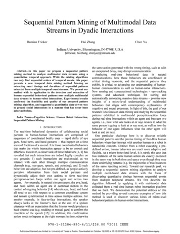
A Temporal Pattern Mining Approach for Classifying Electronic Health Record DataA:3ψ : X X 0 that maps each EHR instance xi to a fixed-size feature vector x0i while preserving the predictive temporal characteristics of xi as much as possible. One approach is to apply astatic transformation and represent the data using a predefined set of features and their values asin [Hauskrecht et al. 2010]. Examples of such features are “most recent creatinine measurement”,“most recent creatinine trend”, “maximum cholesterol measurement”, etc. Our approach is differentand we learn transformation ψ from the data using temporal pattern mining (dynamic transformation). This is done by applying the following steps:(1) Convert the time series variables into a higher level description using temporal abstraction.(2) Mine the minimal predictive temporal patterns Ω.(3) Transform each EHR instance xi to a binary vector x0i , where every feature in x0i correspondsto a specific pattern P Ω and its value is 1 if xi contains P ; and 0 otherwise.After applying this transformation, we can use a standard machine learning method (e.g., SVM,decision tree, naı̈ve Bayes, or logistic regression) on { x0i , yi } to learn function f .3. TEMPORAL PATTERNS FROM ABSTRACTED DATA3.1. Temporal AbstractionThe goal of temporal abstraction [Shahar 1997] is to transform the time series for allclinical variables to a high-level qualitative form. More specifically, each clinical variable(e.g., series of white blood cell counts) is transformed into an interval-based representationhv1 [b1 , e1 ], ., vn [bn , en ]i, where vi Σ is an abstraction that holds from time bi to time ei and Σis the abstraction alphabet that represents a finite set of all permitted abstractions.The most common types of clinical variables in EHR data are: medication administrations andlaboratory results.Medication variables are usually already represented in an interval-based format and specify thetime interval during which a patient was taking a specific medication. For these variables, we simplyuse abstractions that indicate whether the patient is on the medication: Σ {ON, OFF}.Lab variables are usually numerical time series1 that specify the patient’s laboratory results overtime. For these variables, we use two types of temporal abstractions:(1) Trend abstraction that uses the following abstractions: Decreasing (D), Steady (S) and Increasing (I), i.e., Σ {D, S, I}. In our work, we segment the lab series using the sliding windowsegmentation method [Keogh et al. 2003], which keeps expanding each segment until its interpolation error exceeds some error threshold. The abstractions are determined from the slopes ofthe fitted segments. For more information on trend segmentation, see [Keogh et al. 2003].(2) Value abstraction that uses the following abstractions: Very Low (VL), low (L), Normal (N),High (H) and Very High (VH), i.e., Σ {VL, L, N, H, VH}. We use the 10th, 25th, 75th and90th percentiles on the lab values to define these 5 states: a value below the 10th percentile isvery low (VL), a value between the 10th and 25th percentiles is low (L), and so on.Figure 2 shows the trend and value abstractions on a time series of platelet counts of a patient.3.2. State Sequence RepresentationLet a state be an abstraction for a specific variable. For example, state E: Vi D represents adecreasing trend in the values of temporal variable Vi . We sometimes use the shorthand notationDi to denote this state, where the subscript indicates that D is abstracted from the ith variable. Leta state interval be a state that holds during an interval. We denote by (E, bi , ei ) the realization ofstate E in a data instance, where E starts at time bi and ends at time ei .1 Somelab variables may be categorical time series. For example the result of an immunoassay test is either positive ornegative. For such variables, we simply segment the time series into intervals that have the same value.ACM Transactions on Intelligent Systems and Technology, Vol. V, No. N, Article A, Publication date: August 2012.
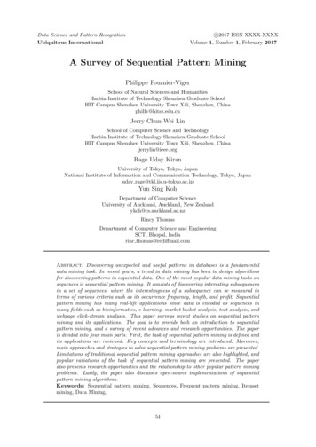
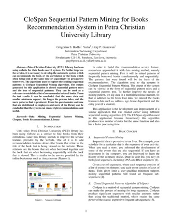
A:4I. Batal et al.Fig. 2. An example illustrating the trend and value abstractions. The blue dashed lines represent the 25th and 75th percentiles and the red solid lines represent the 10th and 90th percentiles.Definition 3.1. A state sequence is a series of state intervals, where the state intervals are ordered according to their start times2 :h(E1 , b1 , e1 ), (E2 , b2 , e2 ), ., (El , bl , el )i: bi ei bi bi 1Note that we do not require ei to be less than bi 1 because the states are obtained from multipletemporal variables and their intervals may overlap.After abstracting all temporal variables, we represent every instance (i.e., patient) in the databaseas a state sequence. We will use the terms instance and state sequence interchangeably hereafter.3.3. Temporal RelationsAllen’s temporal logic [Allen 1984] describes the relations for any pair of state intervals using 13possible relations (see Figure 3). However, it suffices to use the following 7 relations: before, meets,overlaps, is-finished-by, contains, starts and equals because the other relations are simply theirinverses. Allen’s relations have been used by most work on mining time interval data [shan Kamand chee Fu 2000; Hoppner 2003; Papapetrou et al. 2005; Winarko and Roddick 2007; Moskovitchand Shahar 2009].Fig. 3. Allen’s temporal relations.Most of Allen’s relations require equality of one or two of the intervals end points. That is, thereis only a slight difference between overlaps, is-finished-by, contains, starts and equals relations.Hence, when the time information in the data is noisy (not precise), which is the case in EHR data,2 Iftwo interval states have the same start time, we sort them by their end time. If they also have the same end time, we sortthem according to their lexical order.ACM Transactions on Intelligent Systems and Technology, Vol. V, No. N, Article A, Publication date: August 2012.
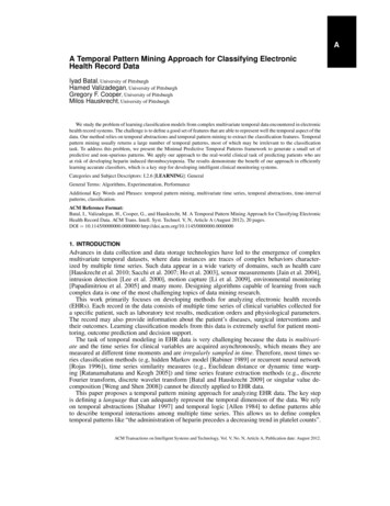
A Temporal Pattern Mining Approach for Classifying Electronic Health Record DataA:5using Allen’s relations may cause the problem of pattern fragmentation [Moerchen 2006]. Thereforewe opt to use only two temporal relations, before (b) and co-occurs (c), which we define as follows:Given two state intervals Ei and Ej :(1) (Ei , bi , ei ) before (Ej , bj , ej ) if ei bj , which is the same as Allen’s before relation.(2) (Ei , bi , ei ) co-occurs with (Ej , bj , ej ), if bi bj ei , i.e. Ei starts before Ej and there is anonempty time period where both Ei and Ej occur.3.4. Temporal PatternsIn order to obtain temporal descriptions of the data, we combine basic states using temporal relations to form temporal patterns. Previously, we saw that the relation between two states can beeither before (b) or co-occurs (c). In order to define relations between k states, we adopt Hoppner’srepresentation of temporal patterns [Hoppner 2003].Definition 3.2. A temporal pattern is defined as P (hS1 , ., Sk i, R), where Si is the ithstate of the pattern and R is an upper triangular matrix that defines the temporal relations betweeneach state and all of its following states:Ri,j Si r Sj :i {1, ., k 1} j {i 1, ., k} r {b, c}The size of pattern P is the number of states it contains. If size(P ) k, we say that P is a k-pattern.Hence, a single state is a 1-pattern (a singleton). We also denote the space of all temporal patternsof arbitrary size by TP.Figure 4 graphically illustrates a 4-pattern with states hA1 , B2 , C3 , B1 i, where thestates are abstractions of temporal variables V1 , V2 and V3 using abstraction alphabetΣ {A, B, C}. The half matrix on the right represents the temporal relations between every stateand the states that follow it. For example, the second state B2 is before the fourth state B1 : R2,4 b.Fig. 4. A temporal pattern with states hA1 , B2 , C3 , B1 i and temporal relations R1,2 c, R1,3 b, R1,4 b,R2,3 c, R2,4 b and R3,4 c.Interesting patterns are usually limited in their temporal extensions, i.e., it would not be interesting to use the before relation to relate states that are temporally very far away from each other.Therefore, the definition of temporal patterns usually comes with a specification of a window sizethat defines the maximum pattern duration [Moerchen 2006; Hoppner 2003; Mannila et al. 1997].In this paper, we are interested in the patient monitoring task, where we have the electronic healthrecord for patient xi up to time ti and we want to decide whether or not patient xi is developinga medical condition that we should alert physicians about. In this task, recent measurements of theclinical variables of xi (close to ti ) are usually more predictive than distant measurements, as wasshown by [Valko and Hauskrecht 2010]. The approach taken in this paper is to define windows offixed width that end at ti for every patient xi and only mine temporal patterns that can be observedinside these windows.Definition 3.3. Let T h(E1 , b1 , e1 ), ., (El , bl , el )i be a state sequence that is visible withina specific window. We say that pattern P (hS1 , ., Sk i, R) occurs in T (or that P covers T ),denoted as P T , if there is an injective mapping π from the states of P to the state intervals of Tsuch that: Si Eπ(i) (Eπ(i) , bπ(i) , eπ(i) ) Ri,j (Eπ(j) , bπ(j) , eπ(j) ) : i {1, ., k} j {i 1, ., k}ACM Transactions on Intelligent Systems and Technology, Vol. V, No. N, Article A, Publication date: August 2012.
A:6I. Batal et al.Notice that checking the existence of a temporal pattern in a state sequence requires: (1) matchingall k states of the patterns and (2) checking that all k(k 1)/2 temporal relations are satisfied.Definition 3.4. P (hS1 , ., Sk1 i, R) is a subpattern of P 0 (hS10 , ., Sk0 2 i, R0 ), denoted asP P 0 , if k1 k2 and there is an injective mapping π from the states of P to the states of P 0 suchthat:00Si Sπ(i) Ri,j Rπ(i),π(j) i {1, ., k1 } j {i 1, ., k1 }For example, pattern (hA1 , C3 i, R1,2 b) is a subpattern of the pattern in Figure 4. If P is asubpattern of P 0 , we say that P 0 is a superpattern of P .Definition 3.5. The support of temporal pattern P in database D is the number of instances inD that contain P :sup(P, D) {Ti : Ti D P Ti } Note that the support definition satisfies the Apriori property [Agrawal and Srikant 1994]: P, P 0 TP if P P 0 sup(P, D) sup(P 0 , D)We define a rule to be of the form P y, where P is a temporal pattern and y is a specific valueof the target class variable Y . We say that rule P y is a subrule of rule P 0 y 0 if P P 0 andy y0 .Definition 3.6. The confidence of rule P y is the proportion of instances from class y in allinstances covered by P :conf (P y) sup(P, Dy )sup(P, D)where Dy denotes all instances in D that belong to class y.Note that the confidence of rule R : P y is the maximum likelihood estimation of the probabilitythat an instance covered by P belongs to class y. If R is a predictive rule of class y, we expect itsconfidence to be larger than the prior probability of y in the data.4. MINING FREQUENT TEMPORAL PATTERNSIn this section, we present our proposed algorithm for mining frequent temporal patterns. We choseto utilize the class information and mine frequent temporal patterns for each class label separatelyusing local minimum supports as opposed to mining frequent temporal patterns from the entire datausing a single global minimum support. The approach is reasonable when pattern mining is appliedin the supervised setting because 1) for unbalanced data, mining frequent patterns using a globalminimum support threshold may result in missing many important patterns in the rare classes and2) mining patterns that are frequent in one of the classes (hence potentially predictive for that class)is more efficient than mining patterns that are globally frequent3 .The mining algorithm takes as input Dy : the state sequences from class y and σy : a user specifiedlocal minimum support threshold. It outputs all frequent temporal patterns in Dy :{P TP : sup(P, Dy ) σy }The mining algorithm performs an Apriori-like level-wise search [Agrawal and Srikant 1994]. Itfirst scans the database to find all frequent 1-patterns. Then for each level k, the algorithm performsthe following two phases to obtain the frequent (k 1)-patterns:3 It is much more efficient to mine patterns that cover more than n instances in one of the classes as opposed to mining allpatterns that cover more than n instances in the entire database (the former is always a subset of the latter).ACM Transactions on Intelligent Systems and Technology, Vol. V, No. N, Article A, Publication date: August 2012.
A Temporal Pattern Mining Approach for Classifying Electronic Health Record DataA:7(1) The candidate generation phase: Generate candidate (k 1)-patterns from the frequent kpatterns.(2) The counting phase: Obtain the frequent (k 1)-patterns by removing candidates with supportless than σy .This process repeats until no more frequent patterns can be found.In the following, we describe in details the candidate generation algorithm and techniques wepropose to improve the efficiency of candidate generation and counting.4.1. Candidate GenerationWe generate a candidate (k 1)-pattern by adding a new state (1-pattern) to the beginning of afrequent k-pattern4 . Let us assume that we are extending pattern P (hS1 , ., Sk i, R) with state0Snew in order to generate candidates of the form (hS10 , ., Sk 1i, R0 ). First of all, we set S10 Snew ,00Si 1 Si for i {1, ., k} and Ri 1,j 1 Ri,j for i {1, ., k 1} j {i 1, ., k}. Thisway, we know that every candidate P 0 of this form is a superpattern of P : P P 0 .In order to fully define a candidate, we still need to specify the temporal relations between the00new state S10 and states S20 , ., Sk 1, i.e., we should define R1,ifor i {2, ., k 1}. Since wehave two possible temporal relations (before and co-occurs), there are 2k possible ways to specifythe missing relations. That is, 2k possible candidates can be generated when adding a new state toa k-pattern. Let L denote all possible states (1-patterns) and let Fk denote the frequent k-patterns,generating the (k 1)-candidates naively in this fashion results in 2k L Fk different candidates.This large number of candidates makes the mining algorithm computationally very expensive andlimits its scalability. Below, we describe the concept of incoherent patterns and introduce a methodthat smartly generates fewer candidates without missing any valid temporal pattern from the result.4.2. Improving the Efficiency of Candidate GenerationDefinition 4.1. A temporal pattern P is incoherent if there does not exist any valid state sequence that contains P .Clearly, we do not have to generate and count incoherent candidates because we know thatthey will have zero support in the dataset. We introduce the following two propositions to avoid0generating incoherent candidates when specifying the relations R1,iin candidates of the form0000P (hS1 , ., Sk 1 i, R ).00P ROPOSITION 4.2. P 0 (hS10 , ., Sk 1i, R0 ) is incoherent if R1,i c and states S10 and Si0belong to the same temporal variable.Two states from the same variable cannot co-occur because temporal abstraction segments eachvariable into non-overlapping state intervals.000P ROPOSITION 4.3. P 0 (hS10 , ., Sk 1i, R0 ) is incoherent if R1,i c j i: R1,j b.P ROOF. Let us assume that there exists a state sequence T h(E1 , b1 , e1 ), ., (El , bl , el )i whereP 0 T . Let π be the mapping from the states of P 0 to the state intervals of T . The definition oftemporal patterns and the fact that state intervals in T are ordered by their start values implies thatthe matching state intervals h(Eπ(1) , bπ(1) , eπ(1) ), ., (Eπ(k 1) , bπ(k 1) , eπ(k 1) )i should also beordered by their start times: bπ(1) . bπ(k 1) . Hence, bπ(j) bπ(i) . We also know that eπ(1) 00bπ(j) because R1,j b. Therefore, eπ(1) bπ(i) . However, since R1,i c, then eπ(1) bπ(i) ,which is a contradiction. Therefore, there is no state sequence that contains P 0 .Example 4.4. Assume we want to extend pattern P (hA1 , B2 , C3 , B1 i, R) in Figure 4 withstate C2 to generate candidates of the form (hC2 , A1 , B2 , C3 , B1 i, R0 ). The relation between the4 Weadd the new state to the beginning of the pattern because this makes the proof of theorem 4.5 easier.ACM Transactions on Intelligent Systems and Technology, Vol. V, No. N, Article A, Publication date: August 2012.
A:8I. Batal et al.00new state C2 and the first state A1 is allowed to be either before or co-occurs: R1,2 b or R1,2 c.However, according to proposition 4.2, C2 cannot co-occur with B2 because they both belong to0temporal variable V2 (R1,36 c). Also, according to proposition 4.3, C2 cannot co-occur with C300(R1,46 c) because C2 is before B2 (R1,3 b) and B2 should start before C3 . For the same reason,0C2 cannot co-occur with B1 (R1,56 c). By removing incoherent patterns, we reduce the numberof candidates that result from adding C2 to 4-pattern P from 24 16 to only 2.T HEOREM 4.5. There are at most k 1 coherent candidates that result from extending a kpattern with a new state.0P ROOF. We know that every candidate P 0 (hS10 , ., Sk 1i, R0 ) corresponds to a specific as0signment of R1,i {b, c} for i 2, .k 1. When we assign the temporal relations, once a relationbecomes before, all the following relations have to be before as well according to proposition 4.3.We can see that the relations can be co-occurs in the beginning of the pattern, but once we see abefore relation at point q {2, ., k 1} in the pattern, all subsequent relations (i q) should bebefore as well:00R1,i c : i {2, ., q 1}; R1,i b : i {q, ., k 1}Therefore, the total number of coherent candidates cannot be more than k 1, which is the totalnumber of different combinations of consecutive co-occurs relations followed by consecutive beforerelations.In some cases, the number of coherent candidates is less than k 1. Assume that there are somestates in P 0 that belong to the same variable as state S10 . Let Sj0 be the first such state (j k 1).0According to proposition 4.2, R1,j6 c. In this case, the number of coherent candidates is j 1 k 1.C OROLLARY 4.6. Let L denote all possible states and let Fk denote all frequent k-patterns. Thenumber of coherent (k 1)-candidates is always less or equal to (k 1) L Fk .So far we described how to generate coherent candidates by appending singletons to the beginning of frequent temporal patterns. However, we do not have to count all coherent candidatesbecause some of them may be guaranteed not to be frequent. To filter out such candidates, we applythe Apriori pruning [Agrawal and Srikant 1994], which removes any candidate (k 1)-pattern if itcontains an infrequent k-subpattern.4.3. Improving the Efficiency of CountingEven after eliminating incoherent candidates and applying the Apriori pruning, the mining algorithmis still computationally expensive because for every candidate, we need to scan the entire databasein the counting phase to check whether or not it is a frequent pattern. The question we try to answerin this section is whether we can omit portions of the database that are guaranteed not to contain thecandidate we want to count. The proposed solution is inspired by [Zaki 2000] that introduced thevertical format for itemset mining and later extended it to sequential pattern mining [Zaki 2001].Let us associate every frequent pattern P with a list of identifiers for all state sequences in Dythat contain P :P.id-list hi1 , i2 , ., in i : Tij Dy P TijClearly, sup(P, Dy ) P.id-list .Definition 4.7. The potential id-list (pid-list) of pattern P is the intersection of the id-listsof its subpatterns:P.pid-list S P S.id-listP ROPOSITION 4.8. P TP : P.id-list P.pid-listACM Transactions on Intelligent Systems and Technology, Vol. V, No. N, Article A, Publication date: August 2012.
A Temporal Pattern Mining Approach for Classifying Electronic Health Record DataA:9P ROOF. Assume Ti is a state sequence in the database such that P Ti . By definition, i P.id-list. We know that Ti must contain all subpatterns of P according to the Apriori property: S P : S Ti . Therefore, S P : i S.id-list i S P S.id-list P.pid-list.Note that for itemset mining, P.pid-list is always equal to P.id-list [Zaki 2000]. However, thisis not true for time-interval temporal patterns. As an example, suppose P (hA1 , B1 , C2 i, R1,2 b, R1,3 b, R2,3 c) and consider the state sequence Ti in Figure 5. Ti contains all subpatterns ofP and hence i P.pid-list. However, Ti does not contain P (there is no mapping π that satisfiesdefinition 3.3); hence i 6 P.id-list.Fig. 5. A state sequence that contains all subpatterns of pattern P (hA1 , B1 , C2 i, R1,2 b, R1,3 b, R2,3 o), butdoes not contain P .Putting it all together, we compute the id-lists in the counting phase (based on the true matches)and the pid-lists in the candidate generation phase. The key idea is that when we count a candidate,we only need to check the state sequences in its pid-list because:i 6 P.pid-list i 6 P.id-list P 6 TiThis offers a lot of computational savings since the pid-lists get smaller as the size of the patternsincreases, making the counting phase much faster.ALGORITHM 1: A high-level description of candidate generation.Input: Frequent k-patterns (Fk )Output: Candidate (k 1)-patterns (Cand) with their pid-lists12345678910111213141516foreach P Fk doforeach I F1 doC generate coherent candidates(P , I);for q 1 to C doS generate k subpatterns(C[q]);if ( S[i] Fk : i {1, ., k} ) thenC[q].pid-list FkS[1] .id-list . FkS[k] .id-list;C[q].mcs max{FkS[1] .mc, ., FkS[k] .mc};if ( C[q].pid-list σy ) thenCand
that mining MPTPs is more efficient than mining all frequent temporal patterns. Our main contributions are summarized as follows: —We propose a novel temporal pattern mining approach for classifying complex EHR data. —We extend our minimal predictive patterns framework [Batal and Hauskrecht 2010] to the tempo-ral domain.