Transcription
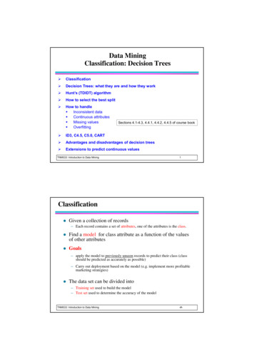
Data MiningClassification: Decision Trees Classification Decision Trees: what they are and how they work Hunt’s (TDIDT) algorithm How to select the best split How to handle Inconsistent data Continuous attributes Missing values OverfittingSections 4.1-4.3, 4.4.1, 4.4.2, 4.4.5 of course book ID3, C4.5, C5.0, CART Advantages and disadvantages of decision trees Extensions to predict continuous valuesTNM033: Introduction to Data Mining1Classification Given a collection of records– Each record contains a set of attributes, one of the attributes is the class. Find a model for class attribute as a function of the valuesof other attributes Goals– apply the model to previously unseen records to predict their class (classshould be predicted as accurately as possible)– Carry out deployment based on the model (e.g. implement more profitablemarketing strategies) The data set can be divided into– Training set used to build the model– Test set used to determine the accuracy of the modelTNM033: Introduction to Data Mining‹#›
Illustrating Classification Attrib1 yes Class NoAttrib1 No Attrib3 95K Class YesTNM033: Introduction to Data Mining‹#›Examples of Classification Task Predicting tumor cells as benign or malignant Classifying credit card transactionsas legitimate or fraudulent Classifying secondary structures of proteinas alpha-helix, beta-sheet, or randomcoil Categorizing news stories as finance,weather, entertainment, sports, etc The UCI Repository of Datasets– http://archive.ics.uci.edu/ml/TNM033: Introduction to Data Mining‹#›
Classification Techniques This lecture introducesDecision Trees Other techniques will be presented in this course:– Rule-based classifiers– But, there are other methods Nearest-neighbor classifiers Naïve Bayes Support-vector machines Neural networksTNM033: Introduction to Data Mining‹#›Example of a Decision TreeTid Refund MaritalStatusTaxableIncome o4YesMarried120KNo5NoDivorced 95KYes6NoMarriedNo7YesDivorced 220K60KSplitting s9NoMarried75KNo10NoSingle90KYesMarriedSingle, Divorced 80KNONO 80KYES10Training DataTNM033: Introduction to Data MiningModel: Decision Tree‹#›
Another Example of Decision TreeTid Refund MaritalStatusTaxableIncome o4YesMarried120KNo5NoDivorced 95KYes6NoMarriedNo7YesDivorced Inc 80K 80KYESNOThere could be more than one tree that fitsthe same data!10Search for the “best tree”TNM033: Introduction to Data Mining‹#›Apply Model to Test DataTest DataStart from the root of tree.RefundYesRefund MaritalStatusTaxableIncome CheatNo80KMarried?10NoNOMarStSingle, DivorcedTaxInc 80KNOTNM033: Introduction to Data MiningMarriedNO 80KYES‹#›
Apply Model to Test DataTest DataRefundYesRefund MaritalStatusTaxableIncome CheatNo80KMarried?10NoNOMarStSingle, DivorcedTaxInc 80KMarriedNO 80KYESNOTNM033: Introduction to Data Mining‹#›Apply Model to Test DataTest DataRefundYesRefund MaritalStatusTaxableIncome CheatNo80KMarried?10NoNOMarStSingle, DivorcedTaxInc 80KNOTNM033: Introduction to Data MiningMarriedNO 80KYES‹#›
Apply Model to Test DataTest DataRefundYesRefund MaritalStatusTaxableIncome CheatNo80KMarried?10NoNOMarStSingle, DivorcedTaxInc 80KMarriedNO 80KYESNOTNM033: Introduction to Data Mining‹#›Apply Model to Test DataTest DataRefundYesRefund MaritalStatusTaxableIncome CheatNo80KMarried?10NoNOMarStSingle, DivorcedTaxInc 80KNOTNM033: Introduction to Data MiningMarriedNO 80KYES‹#›
Apply Model to Test DataTest DataRefundYesRefund MaritalStatusTaxableIncome CheatNo80KMarried?10NoNOMarStMarriedSingle, DivorcedTaxInc 80KAssign Cheat to “No”NO 80KYESNOTNM033: Introduction to Data Mining‹#›Decision Tree Induction How to build a decision tree from a training set?– Many existing systems are based onHunt’s AlgorithmTop-Down Induction of Decision Tree (TDIDT) Employs a top-down search, greedy search through the space ofpossible decision treesTNM033: Introduction to Data Mining‹#›
General Structure of Hunt’s Algorithm Let Dt be the set of training records thatreach a node tGeneral Procedure:– If Dt contains records that belong thesame class yt, then t is a leaf nodelabeled as yt– If Dt contains records that belong tomore than one class, use an attributetest to split the data into smallersubsets. Recursively apply theprocedure to each subsetTid Refund MaritalStatusTaxableIncome o4YesMarried120KNo5NoDivorced 95KYes6NoMarriedNo7YesDivorced es60K10Which attribute should be tested at eachsplitting node?Dt Use some heuristicTNM033: Introduction to Data Mining?Node t‹#›Tree Induction Issues– Determine when to stop splitting– Determine how to split the records Which attribute to use in a split node split?– How to determine the best split? How to specify the attribute test condition?– E.g. X 1? or X Y 1? Shall we use 2-way split or multi-way split?TNM033: Introduction to Data Mining‹#›
Splitting of Nominal Attributes Multi-way split: Use as many partitions as distinctvaluesCarTypeFamilyLuxurySports Binary split: Divides values into two subsets.Need to find optimal y,Luxury}CarTypeTNM033: Introduction to Data Mining{Sports}‹#›Stopping Criteria for Tree Induction Hunt’s algorithm terminates when– All the records in a node belong to the same class– All records in a node have similar attribute values Create a leaf node with the same class label as the majority of thetraining records reaching the node– A minimum pre-specified number of records belong to anodeTNM033: Introduction to Data Mining‹#›
Which Attribute Corresponds to the Best Split?Before Splitting: 10 records of class 0,10 records of class 1Which test condition is the best?(assume the attribute is categorical)TNM033: Introduction to Data Mining‹#›How to determine the Best Split Nodes with homogeneous class distribution arepreferred Need a measure M of node impurity!!Non-homogeneous,Homogeneous,High degree of impurityLow degree of impurityTNM033: Introduction to Data Mining‹#›
Measures of Node Impurity Entropy Gini Index Misclassification errorTNM033: Introduction to Data Mining‹#›How to Find the Best SplitBefore Splitting:C0C1N00N01M0A?B?YesNoNode N1C0C1Node N2N10N11C0C1N20N21M2M1YesNoNode N3C0C1Node N4N30N31C0C1M3M12M4M34GainSplit M0 – M12 vs M0 – M34TNM033: Introduction to Data MiningN40N41‹#›
How to Find the Best SplitBefore Splitting:A?C0C1N00N01M0Node N0YesB?NoNode N1Node N2C0C1C0C1N10N11YesNode N3C0C1N20N21M2M1NoN30N31Node N4C0C1M3N40N41M4Mi Entropy ( Ni ) p ( j Ni ) log p ( j Ni )jTNM033: Introduction to Data Mining‹#›Splitting Criteria Based on Entropy Entropy at a given node t:Entropy (t ) p ( j t ) log p ( j t )j(NOTE: p( j t) is the relative frequency of class j at node t).– Measures homogeneity of a node Maximum (log nc) when records are equally distributed among allclasses implying maximum impurity– nc is the number of classesMinimum (0.0) when all records belong to one class, implying leastimpurityTNM033: Introduction to Data Mining‹#›
Examples for computing EntropyEntropy (t ) p ( j t ) log p ( j t )2jC1C206P(C1) 0/6 0C1C215P(C1) 1/6C1C224P(C1) 2/6P(C2) 6/6 1Entropy – 0 log2 0 – 1 log2 1 – 0 – 0 0P(C2) 5/6Entropy – (1/6) log2 (1/6) – (5/6) log2 (5/6) 0.65P(C2) 4/6Entropy – (2/6) log2 (2/6) – (4/6) log2 (4/6) 0.92TNM033: Introduction to Data Mining‹#›Splitting Based on Information Gain Information Gain:GAIN n Entropy ( p ) Entropy (i ) n ksplitii 1Parent node p with n records is split into k partitions;ni is number of records in partition (node) i– GAINsplit measures Reduction in Entropy achieved because of the splitChoose the split that achieves most reduction (maximizes GAIN) Used in ID3 and C4.5– Disadvantage: bias toward attributes with large number of values Large trees with many branches are preferred What happens if there is an ID attribute?TNM033: Introduction to Data Mining‹#›
Splitting Based on GainRATIO Gain Ratio:GainRATIOsplit GAIN SplitSplitINFOSplitINFO ki 1nnlognniParent node p is split into k partitionsni is the number of records in partition i– GAINsplit is penalized when large number of small partitions areproduced by the split! SplitINFO increases when a larger number of small partitions is producedUsed in C4.5(Ross Quinlan)– Designed to overcome the disadvantage of Information Gain.TNM033: Introduction to Data Mining‹#›Split InformationSplitINFO ki 1nnlognniiA 1A 2A 3A 3: Introduction to Data Mining‹#›i
Other Measures of Impurity Gini Index for a given node t :GINI (t ) 1 [ p ( j t )]2j(NOTE: p( j t) is the relative frequency of class j at node t) Classification error at a node t:Error (t ) 1 max P (i t )iTNM033: Introduction to Data Mining‹#›Comparison among Splitting CriteriaFor a 2-class problem:TNM033: Introduction to Data Mining‹#›
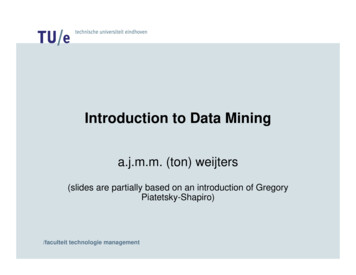
Practical Issues in Learning Decision Trees Conclusion: decision trees are built by greedy searchalgorithms, guided by some heuristic that measures“impurity” In real-world applications we need also to consider– Continuous attributes– Missing values– Improving computational efficiency– Overfitted treesTNM033: Introduction to Data Mining‹#›Splitting of Continuous Attributes Different ways of handling– Discretize once at the beginning– Binary Decision: (A v) or (A v) A is a continuous attribute: consider all possible splits and find thebest cut can be more computational intensiveTNM033: Introduction to Data Mining‹#›
Continuous Attributes Several Choices for the splitting valueTid Refund MaritalStatusTaxableIncome 0KNo4YesMarried120KNo5NoDivorced 95KYes6NoMarriedNo7YesDivorced esFor each splitting value v1.2.3. Scan the data set andCompute class counts in each of thepartitions, A v and A vCompute the entropy/Gini indexChoose the value v that gives lowestentropy/Gini indexRepetition of workEfficient implementation–60K10Naïve algoritm– Number of possible splitting values Number of distinct values nO(n2)TaxableIncomeO(m nlog(n))m is the nunber of attributes and n is thenumber of recordsTNM033: Introduction to Data Mining 85 85‹#›Handling Missing Attribute Values Missing values affect decision tree construction inthree different ways:– Affects how impurity measures are computed– Affects how to distribute instance with missing value tochild nodes How to build a decision tree when some records have missing values?Usually, missing values should be handled during the preprocessing phaseTNM033: Introduction to Data Mining‹#›
Distribute Training Instances with missing valuesTid Refund MaritalStatusTaxableIncome o4YesMarried120KNo5NoDivorced 95KYes6NoMarriedNo7YesDivorced lass Yes0 3/9Class Yes2 6/9Class No3Class No4Send down record Tid 10 tothe left child with weight 3/9 and tothe right child with weight 6/910RefundYesTid RefundNoClass Yes0Cheat Yes2Class No3Cheat No4TNM033: Introduction to Data Mining‹#›Overfitting A tree that fits the training data too well may not be a goodclassifier for new examples.Overfitting results in decision trees more complex thannecessaryEstimating error rates– Use statistical techniques– Re-substitution errors: error on training data set– Generalization errors: error on a testing data set(training error)(test error)Typically, 2/3 of the data set is reserved to model building and 1/3 for errorestimation Disadvantage: less data is available for training Overfitted trees may have a low re-substitution error but a highgeneralization error.TNM033: Introduction to Data Mining‹#›
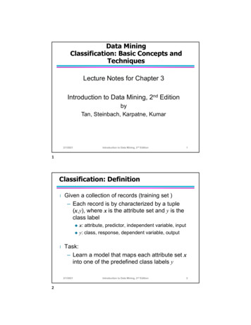
Underfitting and OverfittingOverfittingWhen the tree becomestoo large, its test error ratebegins increasing while itstraining error ratecontinues too decrease.What causes overfitting? NoiseUnderfitting: when model is too simple, both training and test errors are largeTNM033: Introduction to Data Mining‹#›How to Address Overfitting Pre-Pruning (Early Stopping Rule)– Stop the algorithm before it becomes a fully-grown tree Stop if all instances belong to the same class Stop if all the attribute values are the same– Early stopping conditions: Stop if number of instances is less than some user-specified threshold– e.g. 5 to 10 records per node Stop if class distribution of instances are independent of the availableattributes (e.g., using 2 test) Stop if splitting the current node improves the impurity measure (e.g.Gini or information gain) below a given thresholdTNM033: Introduction to Data Mining‹#›
How to Address Overfitting Post-pruning– Grow decision tree to its entirety– Trim the nodes of the decision tree in a bottom-up fashion– Reduced-error pruning Use a dataset not used in the trainingpruning set– Three data sets are needed: training set, test set, pruning set If test error in the pruning set improves after trimming then prunethe tree– Post-pruning can be achieved in two ways:Sub-tree replacement Sub-tree raising See section 4.4.5 of course book TNM033: Introduction to Data Mining‹#›ID3, C4.5, C5.0, CART Ross Quinlan– ID3 uses the Hunt’s algorithm with information gain criterion and gainratio Available in WEKA (no discretization, no missing values)– C4.5 improves ID3 Needs entire data to fit in memory Handles missing attributes and continuous attributes Performs tree post-pruning Available in WEKA as J48– C5.0 is the current commercial successor of C4.5 Breiman et al.– CART builds multivariate decision (binary) trees Available in WEKA as SimpleCARTTNM033: Introduction to Data Mining‹#›
Decision Boundary Border line between two neighboring regions of different classes is known asdecision boundary. Decision boundary is parallel to axes because test condition involves a singleattribute at-a-timeTNM033: Introduction to Data Mining‹#›Oblique Decision Treesx y 1Class Class Test condition may involve multiple attributes (e.g. CART) More expressive representation Finding optimal test condition is computationally expensiveTNM033: Introduction to Data Mining‹#›
Advantages of Decision Trees Extremely fast at classifying unknown records Easy to interpret for small-sized trees Able to handle both continuous and discrete attributes Work well in the presence of redundant attributes If methods for avoiding overfitting are provided then decisiontrees are quite robust in the presence of noise Robust to the effect of outliers Provide a clear indication of which fields are most important forpredictionTNM033: Introduction to Data Mining‹#›Disadvantages of Decision Trees Irrelevant attributes may affect badly the construction of adecision tree– E.g. ID numbers Decision boundaries are rectilinear Small variations in the data can imply that very differentlooking trees are generated A sub-tree can be replicated several times Error-prone with too many classes Not good for predicting the value of a continuous class attribute– This problem is addressed by regression trees and model treesTNM033: Introduction to Data Mining‹#›
Tree ReplicationPQS0R0Q1S0101 Same subtree appears in multiple branchesTNM033: Introduction to Data Mining‹#›
TNM033: Introduction to Data Mining ‹#› Illustrating Classification Task Apply Model Learn Model Tid Attrib1 Attrib2 Attrib3 Class 1 Yes Large 125K No 2 No Medium 100K No 3 No Small 70K No 4 Yes Medium 120K No 5 No Large 95K Yes 6 No Medium 60K No 7 Yes Large 220K No 8 No Small 85K Yes 9 No Medium 75K No 10 No Small 90K Yes