Transcription
Data MiningClassification: Basic Concepts, DecisionTrees, and Model EvaluationLecture Notes for Chapter 4Introduction to Data MiningbyTan, Steinbach, Kumar Tan,Steinbach, KumarIntroduction to Data Mining4/18/20041Classification: DefinitionOGiven a collection of records (training set )– Each record contains a set of attributes, one of theattributes is the class.OOFind a model for class attribute as a functionof the values of other attributes.Goal: previously unseen records should beassigned a class as accurately as possible.– A test set is used to determine the accuracy of themodel. Usually, the given data set is divided intotraining and test sets, with training set used to buildthe model and test set used to validate it. Tan,Steinbach, KumarIntroduction to Data Mining4/18/20042
Illustrating Classification tionLearnModelModel10Training yModelClassDeduction10Test Set Tan,Steinbach, KumarIntroduction to Data Mining4/18/20043Examples of Classification TaskOPredicting tumor cells as benign or malignantOClassifying credit card transactionsas legitimate or fraudulentOClassifying secondary structures of proteinas alpha-helix, beta-sheet, or randomcoilOCategorizing news stories as finance,weather, entertainment, sports, etc Tan,Steinbach, KumarIntroduction to Data Mining4/18/20044
Classification TechniquesDecision Tree based MethodsO Rule-based MethodsO Memory based reasoningO Neural NetworksO Naïve Bayes and Bayesian Belief NetworksO Support Vector MachinesO Tan,Steinbach, KumarIntroduction to Data Mining4/18/20045Example of a Decision TreealalusicicuoorornsiggntteteasclcacacoTid Refund MaritalStatusTaxableIncome o4YesMarried120KNo5NoDivorced 95KYes6NoMarriedNo7YesDivorced 220K60KSplitting AttributesRefundYesNoNOMarStSingle, Single90KYes 80KNOMarriedNO 80KYES10Model: Decision TreeTraining Data Tan,Steinbach, KumarIntroduction to Data Mining4/18/20046
Another Example of Decision Treetecaricgoaltecaricgoalncouoti nussasclTid Refund MaritalStatusTaxableIncome o4YesMarried120KNo5NoDivorced 95KYes6NoMarriedNo7YesDivorced Inc 80K 80KYESNOThere could be more than one tree thatfits the same data!10 Tan,Steinbach, KumarIntroduction to Data Mining4/18/20047Decision Tree Classification InductionLearnModelModel10Training yModelClassDecisionTreeDeduction10Test Set Tan,Steinbach, KumarIntroduction to Data Mining4/18/20048
Apply Model to Test DataTest DataStart from the root of tree.RefundTaxableIncome CheatNo80KMarried?10YesNoNOMarStSingle, DivorcedTaxInc 80KRefund MaritalStatusMarriedNO 80KYESNO Tan,Steinbach, KumarIntroduction to Data Mining4/18/20049Apply Model to Test DataTest DataRefundNoNOMarStSingle, DivorcedTaxIncNO Tan,Steinbach, KumarTaxableIncome CheatNo80KMarried?10Yes 80KRefund MaritalStatusMarriedNO 80KYESIntroduction to Data Mining4/18/200410
Apply Model to Test DataTest DataRefundTaxableIncome CheatNo80KMarried?10YesNoNOMarStSingle, DivorcedTaxInc 80KRefund MaritalStatusMarriedNO 80KYESNO Tan,Steinbach, KumarIntroduction to Data Mining4/18/200411Apply Model to Test DataTest DataRefundNoNOMarStSingle, DivorcedTaxIncNO Tan,Steinbach, KumarTaxableIncome CheatNo80KMarried?10Yes 80KRefund MaritalStatusMarriedNO 80KYESIntroduction to Data Mining4/18/200412
Apply Model to Test DataTest DataRefundTaxableIncome CheatNo80KMarried?10YesNoNOMarStSingle, DivorcedTaxInc 80KRefund MaritalStatusMarriedNO 80KYESNO Tan,Steinbach, KumarIntroduction to Data Mining4/18/200413Apply Model to Test DataTest DataRefundNoNOMarStSingle, DivorcedTaxIncNO Tan,Steinbach, KumarTaxableIncome CheatNo80KMarried?10Yes 80KRefund MaritalStatusMarriedAssign Cheat to “No”NO 80KYESIntroduction to Data Mining4/18/200414
Decision Tree Classification InductionLearnModelModel10Training yModelClassDecisionTreeDeduction10Test Set Tan,Steinbach, KumarIntroduction to Data Mining4/18/200415Decision Tree InductionOMany Algorithms:– Hunt’s Algorithm (one of the earliest)– CART– ID3, C4.5– SLIQ,SPRINT Tan,Steinbach, KumarIntroduction to Data Mining4/18/200416
General Structure of Hunt’s AlgorithmOOLet Dt be the set of training recordsthat reach a node tGeneral Procedure:– If Dt contains records thatbelong the same class yt, then tis a leaf node labeled as yt– If Dt is an empty set, then t is aleaf node labeled by the defaultclass, yd– If Dt contains records thatbelong to more than one class,use an attribute test to split thedata into smaller subsets.Recursively apply theprocedure to each subset. Tan,Steinbach, 20KNo5NoDivorced 95KYes6NoMarriedNo7YesDivorced duction to Data bleIncome Cheat10Hunt’s AlgorithmDon’tCheatTid Refund MaritalStatusNo17Tid Refund MaritalStatusTaxableIncome o4YesMarried120KNo5NoDivorced 95KYes6NoMarriedNo7YesDivorced CheatTaxableIncomeDon’tCheat Tan,Steinbach, KumarMaritalStatus 80K 80KDon’tCheatCheatIntroduction to Data Mining4/18/200418
Tree InductionOGreedy strategy.– Split the records based on an attribute testthat optimizes certain criterion.OIssues– Determine how to split the records Howto specify the attribute test condition? How to determine the best split?– Determine when to stop splitting Tan,Steinbach, KumarIntroduction to Data Mining4/18/200419Tree InductionOGreedy strategy.– Split the records based on an attribute testthat optimizes certain criterion.OIssues– Determine how to split the records Howto specify the attribute test condition? How to determine the best split?– Determine when to stop splitting Tan,Steinbach, KumarIntroduction to Data Mining4/18/200420
How to Specify Test Condition?ODepends on attribute types– Nominal– Ordinal– ContinuousODepends on number of ways to split– 2-way split– Multi-way split Tan,Steinbach, KumarIntroduction to Data Mining4/18/200421Splitting Based on Nominal AttributesOMulti-way split: Use as many partitions as distinctvalues.CarTypeFamilyLuxurySportsOBinary split: Divides values into two subsets.Need to find optimal partitioning.{Sports,Luxury}CarType Tan,Steinbach, Kumar{Family}ORIntroduction to Data Mining{Family,Luxury}CarType{Sports}4/18/200422
Splitting Based on Ordinal AttributesOMulti-way split: Use as many partitions as distinctvalues.SizeSmallLargeMediumOBinary split: Divides values into two subsets.Need to find optimal partitioning.{Small,Medium}OSize{Large}What about this split? Tan,Steinbach, Medium}Introduction to Data Mining4/18/200423Splitting Based on Continuous AttributesODifferent ways of handling– Discretization to form an ordinal categoricalattributeStatic – discretize once at the beginning Dynamic – ranges can be found by equal intervalbucketing, equal frequency bucketing(percentiles), or clustering. – Binary Decision: (A v) or (A v)consider all possible splits and finds the best cut can be more compute intensive Tan,Steinbach, KumarIntroduction to Data Mining4/18/200424
Splitting Based on Continuous AttributesTaxableIncome 80K?TaxableIncome? 10KYes 80KNo[10K,25K)(i) Binary split Tan,Steinbach, Kumar[25K,50K)[50K,80K)(ii) Multi-way splitIntroduction to Data Mining4/18/200425Tree InductionOGreedy strategy.– Split the records based on an attribute testthat optimizes certain criterion.OIssues– Determine how to split the records Howto specify the attribute test condition? How to determine the best split?– Determine when to stop splitting Tan,Steinbach, KumarIntroduction to Data Mining4/18/200426
How to determine the Best SplitBefore Splitting: 10 records of class 0,10 records of class sC0: 6C1: 4C0: 4C1: 6C0: 1C1: 3C0: 8C1: 0C0: 1C1: 7C0: 1C1: 0.c10c11C0: 1C1: 0C0: 0C1: 1c20.C0: 0C1: 1Which test condition is the best? Tan,Steinbach, KumarIntroduction to Data Mining4/18/200427How to determine the Best SplitGreedy approach:– Nodes with homogeneous class distributionare preferredO Need a measure of node impurity:OC0: 5C1: 5C0: 9C1: 1Non-homogeneous,Homogeneous,High degree of impurityLow degree of impurity Tan,Steinbach, KumarIntroduction to Data Mining4/18/200428
Measures of Node ImpurityOGini IndexOEntropyOMisclassification error Tan,Steinbach, KumarIntroduction to Data Mining4/18/200429How to Find the Best SplitBefore Splitting:C0C1N00N01M0A?B?YesNoNode N1C0C1Node N2N10N11C0C1N20N21M2M1YesNoNode N3C0C1Node N4N30N31C0C1M3M12N40N41M4M34Gain M0 – M12 vs M0 – M34 Tan,Steinbach, KumarIntroduction to Data Mining4/18/200430
Measure of Impurity: GINIOGini Index for a given node t :GINI (t ) 1 [ p ( j t )]2j(NOTE: p( j t) is the relative frequency of class j at node t).– Maximum (1 - 1/nc) when records are equallydistributed among all classes, implying leastinteresting information– Minimum (0.0) when all records belong to one class,implying most interesting informationC1C206Gini 0.000 Tan,Steinbach, KumarC1C215C1C2Gini 0.27824Gini 0.444C1C233Gini 0.500Introduction to Data Mining4/18/200431Examples for computing GINIGINI (t ) 1 [ p ( j t )]2jC1C206P(C1) 0/6 0C1C215P(C1) 1/6C1C224P(C1) 2/6 Tan,Steinbach, KumarP(C2) 6/6 1Gini 1 – P(C1)2 – P(C2)2 1 – 0 – 1 0P(C2) 5/6Gini 1 – (1/6)2 – (5/6)2 0.278P(C2) 4/6Gini 1 – (2/6)2 – (4/6)2 0.444Introduction to Data Mining4/18/200432
Splitting Based on GINIOOUsed in CART, SLIQ, SPRINT.When a node p is split into k partitions (children), thequality of split is computed as,kGINI split i 1where,niGINI (i )nni number of records at child i,n number of records at node p. Tan,Steinbach, KumarIntroduction to Data Mining4/18/200433Binary Attributes: Computing GINI IndexOOSplits into two partitionsEffect of Weighing partitions:– Larger and Purer Partitions are sought for.ParentB?YesNoC16C26Gini 0.500Gini(N1) 1 – (5/6)2 – (2/6)2 0.194Gini(N2) 1 – (1/6)2 – (4/6)2 0.528 Tan,Steinbach, KumarNode N1Node N2C1C2N152N214Gini 0.333Introduction to Data MiningGini(Children) 7/12 * 0.194 5/12 * 0.528 0.3334/18/200434
Categorical Attributes: Computing Gini IndexOOFor each distinct value, gather counts for each class inthe datasetUse the count matrix to make decisionsMulti-way splitTwo-way split(find best partition of values)CarTypeC1C2GiniFamily Sports Luxury1214110.393 Tan,Steinbach, 00Introduction to Data 4194/18/200435Continuous Attributes: Computing Gini IndexOOOOUse Binary Decisions based on onevalueSeveral Choices for the splitting value– Number of possible splitting values Number of distinct valuesEach splitting value has a count matrixassociated with it– Class counts in each of thepartitions, A v and A vSimple method to choose best v– For each v, scan the database togather count matrix and computeits Gini index– Computationally Inefficient!Repetition of work. Tan,Steinbach, KumarIntroduction to Data MiningTid Refund MaritalStatusTaxableIncome o4YesMarried120KNo5NoDivorced 95KYes6NoMarriedNo7YesDivorced es60K10TaxableIncome 80K?Yes4/18/2004No36
Continuous Attributes: Computing Gini Index.OFor efficient computation: for each attribute,– Sort the attribute on values– Linearly scan these values, each time updating the count matrixand computing gini index– Choose the split position that has the least gini indexCheatNoNoNoYesYesYesNoNoNoNoTaxable Income60Sorted Values7055Split 230 ini0.420 Tan,Steinbach, on to Data Mining0.3750.4000.4204/18/200437Alternative Splitting Criteria based on INFOOEntropy at a given node t:Entropy (t ) p ( j t ) log p ( j t )j(NOTE: p( j t) is the relative frequency of class j at node t).– Measures homogeneity of a node. Maximum(log nc) when records are equally distributedamong all classes implying least information Minimum (0.0) when all records belong to one class,implying most information– Entropy based computations are similar to theGINI index computations Tan,Steinbach, KumarIntroduction to Data Mining4/18/200438
Examples for computing EntropyEntropy (t ) p ( j t ) log p ( j t )2jC1C206P(C1) 0/6 0C1C215P(C1) 1/6C1C224P(C1) 2/6P(C2) 6/6 1Entropy – 0 log 0 – 1 log 1 – 0 – 0 0P(C2) 5/6Entropy – (1/6) log2 (1/6) – (5/6) log2 (1/6) 0.65P(C2) 4/6Entropy – (2/6) log2 (2/6) – (4/6) log2 (4/6) 0.92 Tan,Steinbach, KumarIntroduction to Data Mining4/18/200439Splitting Based on INFO.OInformation Gain:GAINn Entropy ( p ) Entropy (i ) n ksplitii 1Parent Node, p is split into k partitions;ni is number of records in partition i– Measures Reduction in Entropy achieved because ofthe split. Choose the split that achieves most reduction(maximizes GAIN)– Used in ID3 and C4.5– Disadvantage: Tends to prefer splits that result in largenumber of partitions, each being small but pure. Tan,Steinbach, KumarIntroduction to Data Mining4/18/200440
Splitting Based on INFO.OGain Ratio:GainRATIOsplit GAINnnSplitINFO logSplitINFOnnkSplitiii 1Parent Node, p is split into k partitionsni is the number of records in partition i– Adjusts Information Gain by the entropy of thepartitioning (SplitINFO). Higher entropy partitioning(large number of small partitions) is penalized!– Used in C4.5– Designed to overcome the disadvantage of InformationGain Tan,Steinbach, KumarIntroduction to Data Mining4/18/200441Splitting Criteria based on Classification ErrorOClassification error at a node t :Error (t ) 1 max P (i t )iOMeasures misclassification error made by a node. Maximum(1 - 1/nc) when records are equally distributedamong all classes, implying least interesting information Minimum(0.0) when all records belong to one class, implyingmost interesting information Tan,Steinbach, KumarIntroduction to Data Mining4/18/200442
Examples for Computing ErrorError (t ) 1 max P (i t )iC1C206P(C1) 0/6 0C1C215P(C1) 1/6C1C224P(C1) 2/6 Tan,Steinbach, KumarP(C2) 6/6 1Error 1 – max (0, 1) 1 – 1 0P(C2) 5/6Error 1 – max (1/6, 5/6) 1 – 5/6 1/6P(C2) 4/6Error 1 – max (2/6, 4/6) 1 – 4/6 1/3Introduction to Data Mining4/18/200443Comparison among Splitting CriteriaFor a 2-class problem: Tan,Steinbach, KumarIntroduction to Data Mining4/18/200444
Misclassification Error vs GiniParentA?YesNoNode N1Gini(N1) 1 – (3/3)2 – (0/3)2 0Gini(N2) 1 – (4/7)2 – (3/7)2 0.489 Tan,Steinbach, KumarN130N243Gini 0.3617C23Gini 0.42Node N2C1C2C1Gini(Children) 3/10 * 0 7/10 * 0.489 0.342Gini improves !!Introduction to Data Mining4/18/200445Tree InductionOGreedy strategy.– Split the records based on an attribute testthat optimizes certain criterion.OIssues– Determine how to split the records Howto specify the attribute test condition? How to determine the best split?– Determine when to stop splitting Tan,Steinbach, KumarIntroduction to Data Mining4/18/200446
Stopping Criteria for Tree InductionOStop expanding a node when all the recordsbelong to the same classOStop expanding a node when all the records havesimilar attribute valuesOEarly termination (to be discussed later) Tan,Steinbach, KumarIntroduction to Data Mining4/18/200447Decision Tree Based ClassificationOAdvantages:– Inexpensive to construct– Extremely fast at classifying unknown records– Easy to interpret for small-sized trees– Accuracy is comparable to other classificationtechniques for many simple data sets Tan,Steinbach, KumarIntroduction to Data Mining4/18/200448
Example: C4.5Simple depth-first construction.O Uses Information GainO Sorts Continuous Attributes at each node.O Needs entire data to fit in memory.O Unsuitable for Large Datasets.– Needs out-of-core sorting.OOYou can download the software from:http://www.cse.unsw.edu.au/ quinlan/c4.5r8.tar.gz Tan,Steinbach, KumarIntroduction to Data Mining4/18/200449Practical Issues of ClassificationOUnderfitting and OverfittingOMissing ValuesOCosts of Classification Tan,Steinbach, KumarIntroduction to Data Mining4/18/200450
Underfitting and Overfitting (Example)500 circular and 500triangular data points.Circular points:0.5 sqrt(x12 x22) 1Triangular points:sqrt(x12 x22) 0.5 orsqrt(x12 x22) 1 Tan,Steinbach, KumarIntroduction to Data Mining4/18/200451Underfitting and OverfittingOverfittingUnderfitting: when model is too simple, both training and test errors are large Tan,Steinbach, KumarIntroduction to Data Mining4/18/200452
Overfitting due to NoiseDecision boundary is distorted by noise point Tan,Steinbach, KumarIntroduction to Data Mining4/18/200453Overfitting due to Insufficient ExamplesLack of data points in the lower half of the diagram makes it difficultto predict correctly the class labels of that region- Insufficient number of training records in the region causes thedecision tree to predict the test examples using other trainingrecords that are irrelevant to the classification task Tan,Steinbach, KumarIntroduction to Data Mining4/18/200454
Notes on OverfittingOOverfitting results in decision trees that are morecomplex than necessaryOTraining error no longer provides a good estimateof how well the tree will perform on previouslyunseen recordsONeed new ways for estimating errors Tan,Steinbach, KumarIntroduction to Data Mining4/18/200455Estimating Generalization ErrorsOOORe-substitution errors: error on training (Σ e(t) )Generalization errors: error on testing (Σ e’(t))Methods for estimating generalization errors:– Optimistic approach: e’(t) e(t)– Pessimistic approach: For each leaf node: e’(t) (e(t) 0.5)Total errors: e’(T) e(T) N 0.5 (N: number of leaf nodes)For a tree with 30 leaf nodes and 10 errors on training(out of 1000 instances):Training error 10/1000 1%Generalization error (10 30 0.5)/1000 2.5%– Reduced error pruning (REP): uses validation data set to estimate generalizationerror Tan,Steinbach, KumarIntroduction to Data Mining4/18/200456
Occam’s RazorOGiven two models of similar generalization errors,one should prefer the simpler model over themore complex modelOFor complex models, there is a greater chancethat it was fitted accidentally by errors in dataOTherefore, one should include model complexitywhen evaluating a model Tan,Steinbach, KumarIntroduction to Data Mining4/18/200457Minimum Description Length (MDL)OOOXX1X2X3X4y1001 Xn1A?YesNo0B?B2B1AC?1C1C201BXX1X2X3X4y? Xn?Cost(Model,Data) Cost(Data Model) Cost(Model)– Cost is the number of bits needed for encoding.– Search for the least costly model.Cost(Data Model) encodes the misclassification errors.Cost(Model) uses node encoding (number of children)plus splitting condition encoding. Tan,Steinbach, KumarIntroduction to Data Mining4/18/200458
How to Address OverfittingOPre-Pruning (Early Stopping Rule)– Stop the algorithm before it becomes a fully-grown tree– Typical stopping conditions for a node: Stop if all instances belong to the same class Stop if all the attribute values are the same– More restrictive conditions: Stop if number of instances is less than some user-specifiedthreshold Stop if class distribution of instances are independent of theavailable features (e.g., using χ 2 test) Stop if expanding the current node does not improve impuritymeasures (e.g., Gini or information gain). Tan,Steinbach, KumarIntroduction to Data Mining4/18/200459How to Address Overfitting OPost-pruning– Grow decision tree to its entirety– Trim the nodes of the decision tree in abottom-up fashion– If generalization error improves after trimming,replace sub-tree by a leaf node.– Class label of leaf node is determined frommajority class of instances in the sub-tree– Can use MDL for post-pruning Tan,Steinbach, KumarIntroduction to Data Mining4/18/200460
Example of Post-PruningTraining Error (Before splitting) 10/30Class Yes20Pessimistic error (10 0.5)/30 10.5/30Class No10Training Error (After splitting) 9/30Pessimistic error (After splitting)Error 10/30 (9 4 0.5)/30 11/30PRUNE!A?A1A4A3A2Class Yes8Class Yes3Class Yes4Class Yes5Class No4Class No4Class No1Class No1 Tan,Steinbach, KumarIntroduction to Data Mining4/18/200461Examples of Post-pruning– Optimistic error?Case 1:Don’t prune for both cases– Pessimistic error?C0: 11C1: 3C0: 2C1: 4C0: 14C1: 3C0: 2C1: 2Don’t prune case 1, prune case 2– Reduced error pruning?Case 2:Depends on validation set Tan,Steinbach, KumarIntroduction to Data Mining4/18/200462
Handling Missing Attribute ValuesOMissing values affect decision tree construction inthree different ways:– Affects how impurity measures are computed– Affects how to distribute instance with missingvalue to child nodes– Affects how a test instance with missing valueis classified Tan,Steinbach, KumarIntroduction to Data Mining4/18/200463Computing Impurity MeasureBefore Splitting:Entropy(Parent) -0.3 log(0.3)-(0.7)log(0.7) 0.8813Tid Refund MaritalStatusTaxableIncome o4YesMarried120KNo5NoDivorced 95KYes6NoMarriedNo7YesDivorced 220KNo8NoSingle85KYesEntropy(Refund Yes) 09NoMarried75KNo10?Single90KYesEntropy(Refund No) -(2/6)log(2/6) – (4/6)log(4/6) 0.918360KRefund YesRefund NoRefund ?Class Class Yes No032410Split on Refund:10Missingvalue Tan,Steinbach, KumarEntropy(Children) 0.3 (0) 0.6 (0.9183) 0.551Gain 0.9 (0.8813 – 0.551) 0.3303Introduction to Data Mining4/18/200464
Distribute InstancesTid Refund MaritalStatusTaxableIncome o4YesMarried120KNo5NoDivorced 95KYes6NoMarriedNo7YesDivorced gle?RefundYesYesNoClass Yes0 3/9Class Yes2 6/9Class No3Class No4Probability that Refund Yes is 3/9Probability that Refund No is 6/9NoClass Yes0Cheat Yes2Class No3Cheat No4 Tan,Steinbach, KumarTaxableIncome Class1010RefundTid Refund MaritalStatusAssign record to the left child withweight 3/9 and to the right childwith weight 6/9Introduction to Data Mining4/18/200465Classify InstancesNew record:MarriedTid Refund MaritalStatusTaxableIncome Class1185KNo?10RefundYesNOSingleDivorced TotalClass No3104Class arriedTaxInc 80KNO Tan,Steinbach, KumarNO 80KProbability that Marital Status Married is 3.67/6.67Probability that Marital Status {Single,Divorced} is 3/6.67YESIntroduction to Data Mining4/18/200466
Other IssuesData FragmentationO Search StrategyO ExpressivenessO Tree ReplicationO Tan,Steinbach, KumarIntroduction to Data Mining4/18/200467Data FragmentationONumber of instances gets smaller as you traversedown the treeONumber of instances at the leaf nodes could betoo small to make any statistically significantdecision Tan,Steinbach, KumarIntroduction to Data Mining4/18/200468
Search StrategyOFinding an optimal decision tree is NP-hardOThe algorithm presented so far uses a greedy,top-down, recursive partitioning strategy toinduce a reasonable solutionOOther strategies?– Bottom-up– Bi-directional Tan,Steinbach, KumarIntroduction to Data Mining4/18/200469ExpressivenessODecision tree provides expressive representation forlearning discrete-valued function– But they do not generalize well to certain types ofBoolean functions Example: parity function:– Class 1 if there is an even number of Boolean attributes with truthvalue True– Class 0 if there is an odd number of Boolean attributes with truthvalue True OFor accurate modeling, must have a complete treeNot expressive enough for modeling continuous variables– Particularly when test condition involves only a singleattribute at-a-time Tan,Steinbach, KumarIntroduction to Data Mining4/18/200470
Decision Boundary10.9x 0.43?0.8Yes0.7Noy0.6y 0.33?y 70.80.9NoYes:0:4No:0:3:4:01 Border line between two neighboring regions of different classes isknown as decision boundary Decision boundary is parallel to axes because test condition involvesa single attribute at-a-time Tan,Steinbach, KumarIntroduction to Data Mining4/18/200471Oblique Decision Treesx y 1Class Class Test condition may involve multiple attributes More expressive representation Finding optimal test condition is computationally expensive Tan,Steinbach, KumarIntroduction to Data Mining4/18/200472
Tree ReplicationPQS0R0Q1S0101 Same subtree appears in multiple branches Tan,Steinbach, KumarIntroduction to Data Mining4/18/200473Model EvaluationOMetrics for Performance Evaluation– How to evaluate the performance of a model?OMethods for Performance Evaluation– How to obtain reliable estimates?OMethods for Model Comparison– How to compare the relative performanceamong competing models? Tan,Steinbach, KumarIntroduction to Data Mining4/18/200474
Model EvaluationOMetrics for Performance Evaluation– How to evaluate the performance of a model?OMethods for Performance Evaluation– How to obtain reliable estimates?OMethods for Model Comparison– How to compare the relative performanceamong competing models? Tan,Steinbach, KumarIntroduction to Data Mining4/18/200475Metrics for Performance EvaluationFocus on the predictive capability of a model– Rather than how fast it takes to classify orbuild models, scalability, etc.O Confusion Matrix:OPREDICTED CLASSClass YesClass YesACTUALCLASS Class No Tan,Steinbach, KumarClass NoabcdIntroduction to Data Mininga: TP (true positive)b: FN (false negative)c: FP (false positive)d: TN (true negative)4/18/200476
Metrics for Performance Evaluation PREDICTED CLASSClass YesACTUALCLASSOClass NoClass Yesa(TP)b(FN)Class Noc(FP)d(TN)Most widely-used metric:Accuracy Tan,Steinbach, Kumara dTP TN a b c d TP TN FP FNIntroduction to Data Mining4/18/200477Limitation of AccuracyOConsider a 2-class problem– Number of Class 0 examples 9990– Number of Class 1 examples 10OIf model predicts everything to be class 0,accuracy is 9990/10000 99.9 %– Accuracy is misleading because model doesnot detect any class 1 example Tan,Steinbach, KumarIntroduction to Data Mining4/18/200478
Cost MatrixPREDICTED CLASSClass Yes Class NoC(i j)Class YesACTUALCLASS Class NoC(Yes Yes)C(No Yes)C(Yes No)C(No No)C(i j): Cost of misclassifying class j example as class i Tan,Steinbach, KumarIntroduction to Data Mining4/18/200479Computing Cost of ClassificationCostMatrixPREDICTED CLASSACTUALCLASSModelM1C(i j) - -1100-10PREDICTED CLASS ACTUALCLASSPREDICTED CLASS- 15040-60250Accuracy 80%Cost 3910 Tan,Steinbach, KumarModelM2ACTUALCLASS - 25045-5200Accuracy 90%Cost 4255Introduction to Data Mining4/18/200480
Cost vs AccuracyAccuracy is proportional to cost if1. C(Yes No) C(No Yes) q2. C(Yes Yes) C(No No) pPREDICTED CLASSCountClass YesACTUALCLASSClass NoClass YesabClass NocdN a b c dAccuracy (a d)/NPREDICTED CLASSCostClass YesACTUALCLASSClass YespqClass Noqp Tan,Steinbach, KumarCost p (a d) q (b c)Class No p (a d) q (N – a – d) q N – (q – p)(a d) N [q – (q-p) Accuracy]Introduction to Data Mining4/18/200481Cost-Sensitive MeasuresPrecision (p) Recall (r) aa caa bF - measure (F) OOO2rp2a r p 2a b cPrecision is biased towards C(Yes Yes) & C(Yes No)Recall is biased towards C(Yes Yes) & C(No Yes)F-measure is biased towards all except C(No No)Weighted Accuracy wa w dwa wb wc w d1 Tan,Steinbach, KumarIntroduction to Data Mining142344/18/200482
Model EvaluationOMetrics for Performance Evaluation– How to evaluate the performance of a model?OMethods for Performance Evaluation– How to obtain reliable estimates?OMethods for Model Comparison– How to compare the relative performanceamong competing models? Tan,Steinbach, KumarIntroduction to Data Mining4/18/200483Methods for Performance EvaluationOHow to obtain a reliable estimate ofperformance?OPerformance of a model may depend on otherfactors besides the learning algorithm:– Class distribution– Cost of misclassification– Size of training and test sets Tan,Steinbach, KumarIntroduction to Data Mining4/18/200484
Learning CurveOLearning curve showshow accuracy changeswith varying sample sizeORequires a samplingschedule for creatinglearning curve:OArithmetic sampling(Langley, et al)OGeometric sampling(Provost et al)Effect of small sample size: Tan,Steinbach, KumarIntroduction to Dat
Data Mining Classification: Basic Concepts, Decision Trees, and Model Evaluation Lecture Notes for Chapter 4 Introduction to Data Mining by Tan, Steinbach, Kumar