Transcription
On Market-Making and Delta-Hedging1 Market Makers2 Market-Making and Bond-Pricing
On Market-Making and Delta-Hedging1 Market Makers2 Market-Making and Bond-Pricing
What to market makers do? Provide immediacy by standing ready to sell to buyers (at askprice) and to buy from sellers (at bid price) Generate inventory as needed by short-selling Profit by charging the bid-ask spread Their position is determined by the order flow from customers In contrast, proprietary trading relies on an investment strategy tomake a profit
What to market makers do? Provide immediacy by standing ready to sell to buyers (at askprice) and to buy from sellers (at bid price) Generate inventory as needed by short-selling Profit by charging the bid-ask spread Their position is determined by the order flow from customers In contrast, proprietary trading relies on an investment strategy tomake a profit
What to market makers do? Provide immediacy by standing ready to sell to buyers (at askprice) and to buy from sellers (at bid price) Generate inventory as needed by short-selling Profit by charging the bid-ask spread Their position is determined by the order flow from customers In contrast, proprietary trading relies on an investment strategy tomake a profit
What to market makers do? Provide immediacy by standing ready to sell to buyers (at askprice) and to buy from sellers (at bid price) Generate inventory as needed by short-selling Profit by charging the bid-ask spread Their position is determined by the order flow from customers In contrast, proprietary trading relies on an investment strategy tomake a profit
What to market makers do? Provide immediacy by standing ready to sell to buyers (at askprice) and to buy from sellers (at bid price) Generate inventory as needed by short-selling Profit by charging the bid-ask spread Their position is determined by the order flow from customers In contrast, proprietary trading relies on an investment strategy tomake a profit
Market Maker Risk Market makers attempt to hedge in order to avoid the risk fromtheir arbitrary positions due to customer orders (see Table 13.1 inthe textbook) Option positions can be hedged using delta-hedging Delta-hedged positions should expect to earn risk-free return
Market Maker Risk Market makers attempt to hedge in order to avoid the risk fromtheir arbitrary positions due to customer orders (see Table 13.1 inthe textbook) Option positions can be hedged using delta-hedging Delta-hedged positions should expect to earn risk-free return
Market Maker Risk Market makers attempt to hedge in order to avoid the risk fromtheir arbitrary positions due to customer orders (see Table 13.1 inthe textbook) Option positions can be hedged using delta-hedging Delta-hedged positions should expect to earn risk-free return
Delta and Gamma as measures ofexposure Suppose that Delta is 0.5824, when S 40 (same as in Table 13.1and Figure 13.1) A 0.75 increase in stock price would be expected to increaseoption value by 0.4368 (incerase in price Delta 0.75 x 0.5824) The actual increase in the options value is higher: 0.4548 This is because the Delta increases as stock price increases. Usingthe smaller Delta at the lower stock price understates the theactual change Similarly, using the original Delta overstates the change in theoption value as a response to a stock price decline Using Gamma in addition to Delta improves the approximation ofthe option value change (Since Gamma measures the change inDelta as the stock price varies - it’s like adding another term in theTaylor expansion)
Delta and Gamma as measures ofexposure Suppose that Delta is 0.5824, when S 40 (same as in Table 13.1and Figure 13.1) A 0.75 increase in stock price would be expected to increaseoption value by 0.4368 (incerase in price Delta 0.75 x 0.5824) The actual increase in the options value is higher: 0.4548 This is because the Delta increases as stock price increases. Usingthe smaller Delta at the lower stock price understates the theactual change Similarly, using the original Delta overstates the change in theoption value as a response to a stock price decline Using Gamma in addition to Delta improves the approximation ofthe option value change (Since Gamma measures the change inDelta as the stock price varies - it’s like adding another term in theTaylor expansion)
Delta and Gamma as measures ofexposure Suppose that Delta is 0.5824, when S 40 (same as in Table 13.1and Figure 13.1) A 0.75 increase in stock price would be expected to increaseoption value by 0.4368 (incerase in price Delta 0.75 x 0.5824) The actual increase in the options value is higher: 0.4548 This is because the Delta increases as stock price increases. Usingthe smaller Delta at the lower stock price understates the theactual change Similarly, using the original Delta overstates the change in theoption value as a response to a stock price decline Using Gamma in addition to Delta improves the approximation ofthe option value change (Since Gamma measures the change inDelta as the stock price varies - it’s like adding another term in theTaylor expansion)
Delta and Gamma as measures ofexposure Suppose that Delta is 0.5824, when S 40 (same as in Table 13.1and Figure 13.1) A 0.75 increase in stock price would be expected to increaseoption value by 0.4368 (incerase in price Delta 0.75 x 0.5824) The actual increase in the options value is higher: 0.4548 This is because the Delta increases as stock price increases. Usingthe smaller Delta at the lower stock price understates the theactual change Similarly, using the original Delta overstates the change in theoption value as a response to a stock price decline Using Gamma in addition to Delta improves the approximation ofthe option value change (Since Gamma measures the change inDelta as the stock price varies - it’s like adding another term in theTaylor expansion)
Delta and Gamma as measures ofexposure Suppose that Delta is 0.5824, when S 40 (same as in Table 13.1and Figure 13.1) A 0.75 increase in stock price would be expected to increaseoption value by 0.4368 (incerase in price Delta 0.75 x 0.5824) The actual increase in the options value is higher: 0.4548 This is because the Delta increases as stock price increases. Usingthe smaller Delta at the lower stock price understates the theactual change Similarly, using the original Delta overstates the change in theoption value as a response to a stock price decline Using Gamma in addition to Delta improves the approximation ofthe option value change (Since Gamma measures the change inDelta as the stock price varies - it’s like adding another term in theTaylor expansion)
Delta and Gamma as measures ofexposure Suppose that Delta is 0.5824, when S 40 (same as in Table 13.1and Figure 13.1) A 0.75 increase in stock price would be expected to increaseoption value by 0.4368 (incerase in price Delta 0.75 x 0.5824) The actual increase in the options value is higher: 0.4548 This is because the Delta increases as stock price increases. Usingthe smaller Delta at the lower stock price understates the theactual change Similarly, using the original Delta overstates the change in theoption value as a response to a stock price decline Using Gamma in addition to Delta improves the approximation ofthe option value change (Since Gamma measures the change inDelta as the stock price varies - it’s like adding another term in theTaylor expansion)
On Market-Making and Delta-Hedging1 Market Makers2 Market-Making and Bond-Pricing
Outline The Black model is a version of the Black-Scholes model for whichthe underlying asset is a futures contract We will begin by seeing how the Black model can be used to pricebond and interest rate options Finally, we examine binomial interest rate models, in particular theBlack-Derman-Toy model
Outline The Black model is a version of the Black-Scholes model for whichthe underlying asset is a futures contract We will begin by seeing how the Black model can be used to pricebond and interest rate options Finally, we examine binomial interest rate models, in particular theBlack-Derman-Toy model
Outline The Black model is a version of the Black-Scholes model for whichthe underlying asset is a futures contract We will begin by seeing how the Black model can be used to pricebond and interest rate options Finally, we examine binomial interest rate models, in particular theBlack-Derman-Toy model
Bond Pricing A bond portfolio manager might want to hedge bonds of oneduration with bonds of a different duration. This is called durationhedging. In general, hedging a bond portfolio based on durationdoes not result in a perfect hedge We focus on zero-coupon bonds (as they are components of morecomplicated instruments)
Bond Pricing A bond portfolio manager might want to hedge bonds of oneduration with bonds of a different duration. This is called durationhedging. In general, hedging a bond portfolio based on durationdoes not result in a perfect hedge We focus on zero-coupon bonds (as they are components of morecomplicated instruments)
The Dynamics of Bonds and Interest Rates Suppose that the bond-price at time T t before maturity isdenoted by P(t, T ) and that it is modeled by the following Itoprocess:dPt α(r , t) dt q(r , t) dZtPtwhere12Z is a standard Brownian motionα and q are coefficients which depend both on time t and theinterest rate r This aproach requires careful specificatio of the coefficients α and q- and we would like for the model to be simpler . The alternative is to start with the model of the short-term interestrate as an Ito process:dr a(r ) dt σ(r ) dZand continue to price the bonds by solving for the bond price
The Dynamics of Bonds and Interest Rates Suppose that the bond-price at time T t before maturity isdenoted by P(t, T ) and that it is modeled by the following Itoprocess:dPt α(r , t) dt q(r , t) dZtPtwhere12Z is a standard Brownian motionα and q are coefficients which depend both on time t and theinterest rate r This aproach requires careful specificatio of the coefficients α and q- and we would like for the model to be simpler . The alternative is to start with the model of the short-term interestrate as an Ito process:dr a(r ) dt σ(r ) dZand continue to price the bonds by solving for the bond price
The Dynamics of Bonds and Interest Rates Suppose that the bond-price at time T t before maturity isdenoted by P(t, T ) and that it is modeled by the following Itoprocess:dPt α(r , t) dt q(r , t) dZtPtwhere12Z is a standard Brownian motionα and q are coefficients which depend both on time t and theinterest rate r This aproach requires careful specificatio of the coefficients α and q- and we would like for the model to be simpler . The alternative is to start with the model of the short-term interestrate as an Ito process:dr a(r ) dt σ(r ) dZand continue to price the bonds by solving for the bond price
An Inappropriate Bond-Pricing Model We need to be careful when implementing the above strategy. For instance, if we assume that the yield-curve is flat, i.e., that atany time the zero-coupon bonds at all maturities have the sameyield to maturity, we get that there is possibility for arbitrage The construction of the portfolio which creates arbitrage is similar tothe one for different Sharpe Ratios and a single source ofuncertainty. You should read Section 24.1
An Inappropriate Bond-Pricing Model We need to be careful when implementing the above strategy. For instance, if we assume that the yield-curve is flat, i.e., that atany time the zero-coupon bonds at all maturities have the sameyield to maturity, we get that there is possibility for arbitrage The construction of the portfolio which creates arbitrage is similar tothe one for different Sharpe Ratios and a single source ofuncertainty. You should read Section 24.1
An Inappropriate Bond-Pricing Model We need to be careful when implementing the above strategy. For instance, if we assume that the yield-curve is flat, i.e., that atany time the zero-coupon bonds at all maturities have the sameyield to maturity, we get that there is possibility for arbitrage The construction of the portfolio which creates arbitrage is similar tothe one for different Sharpe Ratios and a single source ofuncertainty. You should read Section 24.1
An Equilibrium Equation for Bonds When the short-term interest rate is the only source of uncertainty,the following partial differential equation must be satisfied by anyzero-coupon bond (see equation (24.18) in the textbook)1 2P P Pσ(r )2 2 [α(r ) σ(r )φ(r , t)] rP 02 r r twhere1r denotes the short-term interest rate, which follows the Ito processdr a(r )dt σ(r )dZ ;2φ(r , t) is the Sharpe ratio corresponding to the source of uncertaintyZ , i.e.,φ(r , t) α(r , t, T ) rq(r , t, T )with the coefficients P · α and P · q are the drift and the volatility(respectively) of the Ito process P which represents the bond-pricefor the interest-rate r This equation characterizes claims that are a function of the interestrate (as there are no alternative sources of uncertainty).
An Equilibrium Equation for Bonds When the short-term interest rate is the only source of uncertainty,the following partial differential equation must be satisfied by anyzero-coupon bond (see equation (24.18) in the textbook)1 2P P Pσ(r )2 2 [α(r ) σ(r )φ(r , t)] rP 02 r r twhere1r denotes the short-term interest rate, which follows the Ito processdr a(r )dt σ(r )dZ ;2φ(r , t) is the Sharpe ratio corresponding to the source of uncertaintyZ , i.e.,φ(r , t) α(r , t, T ) rq(r , t, T )with the coefficients P · α and P · q are the drift and the volatility(respectively) of the Ito process P whic
option value by 0.4368 (incerase in price Delta 0.75 x 0.5824) The actual increase in the options value is higher: 0.4548 This is because the Delta increases as stock price increases.