WIXLIB

Optimal High-Frequency Market MakingTakahiro Fushimi, Christian González Rojas,and Molly Herman{tfushimi, cgrojas, mrherman}@stanford.eduJune 11, 2018AbstractThe paper implements and analyzes the high frequency market making pricingmodel by Avellaneda and Stoikov (2008). This pricing model is integrated with aproprietary inventory control model that dynamically adjusts the order size to mitigateinventory risk, the risk that we bear due to our inventory. Then, we develop a tradingsimulator to assess the P&L and inventory of our optimal pricing strategy in comparison to a baseline pricing model for five representative stocks. With the inventorymodel, the optimal pricing model outperforms the baseline in inventory managementwhile ensuring profitability.Contents1 Introduction22 Market Making Model22.12.22.3Pricing . . . . . . . . . . . . . . . . . . . . . . . . . . . . . . . . . . . . . . .Inventory . . . . . . . . . . . . . . . . . . . . . . . . . . . . . . . . . . . . .Algorithm . . . . . . . . . . . . . . . . . . . . . . . . . . . . . . . . . . . . .3 Trading Simulator3.13.26Market Order Dynamics . . . . . . . . . . . . . . . . . . . . . . . . . . . . .Order Execution . . . . . . . . . . . . . . . . . . . . . . . . . . . . . . . . .4 Experiments4.14.2345677Results . . . . . . . . . . . . . . . . . . . . . . . . . . . . . . . . . . . . . . .Markov Chain Analysis . . . . . . . . . . . . . . . . . . . . . . . . . . . . . .7115 Conclusions12References131

1IntroductionMarket makers are critical providers of liquidity in markets as they constantly place bid andask orders in the limit order book such that any market order will always be capable of beingfilled. The goal of the market maker is to strategically place these bids and asks to capture thespread, the difference between the bid and ask price, while also earning a rebate for providingliquidity. On the other hand, market making has become one of the prevailing strategies forhigh-frequency traders who profit by turning over positions in an extremely short period.These high-frequency traders play integral roles in providing liquidity to markets, accountingfor more than 50% of total volume in the US-listed equities (SEC, 2014).Various pricing models for market making have been proposed in the academic literature. Hoand Stoll (1981) is one of the early studies that analyze the market making problem under astochastic control framework. Avellaneda and Stoikov (2008) extends the model proposed byHo and Stoll (1981), derives the optimal bid and ask quotes using asymptotic expansion andapplies it to high-frequency market making. Furthermore, Guéant, Lehalle, and FernandezTapia (2013) develops the model further by deriving the closed form solution of the optimalbid and ask spread with boundary conditions on inventory size.In this paper, we implement the high frequency market making pricing model proposedby Avellaneda and Stoikov (2008). We choose this model for the ease of implementationand analysis, and unlike recent models such as Guéant et al. (2013), it does not restrict thepermissible inventory size. Although this unconstrained inventory assumption lets the marketmaker to keep trading regardless of their position, it is a shortcoming since it increases thelikelihood of accumulating a one-sided position and getting exposed to inventory risk, the riskthat we bear due to inventory. To complement the pricing model, we develop an inventorycontrol model that dynamically adjusts the order size based on the current position. Thisintegrated approach allows us to effectively control inventory risk while ensuring profitability.A trading simulator is devised to assess the P&L and inventory of our optimal pricing strategycompared to a baseline pricing model for five representative stocks.The rest of the paper is organized as follows: Section 2 describes the pricing model andthe inventory model, section 3 explains a trading simulator on which the strategy is tested,section 4 discusses the experiment and results, while section 5 concludes.2Market Making ModelAs a high-frequency market maker, we integrate the pricing framework proposed by Avellanedaand Stoikov (2008) and a proprietary order size dynamic model. The combination of an optimal quote and a dynamic order size strategy allows us to effectively control inventory riskand ensure profitability.2

2.1PricingWe use the optimal market making model developed by Avellaneda and Stoikov (2008) as ourbid and ask quote-setting strategy. The framework is based on a utility-maximizing marketmaker trading in a limit order book. This section presents a brief summary of the model.We are interested in maximizing our expected exponential utility given our profit and loss atterminal time T . Assuming the risk-free rate is zero and the mid-price of a stock follows astandard brownian motion dSt σdWt with initial value S0 s and standard deviation σ,Avellaneda and Stoikov (2008) formulates the market maker problem as: u(s, x, q, t) max Et e γ(XT qT ST )δ a ,δ bwhere δ a , δ b are the bid and ask spreadsγ is a risk aversion parameterXT is the cash at time TqT is the inventory at time TST is the stock price at time TA few assumptions must be made before solving the stochastic optimal control problem.First, it is important to model inventory as a stochastic process, given that order fills arerandom variables. Therefore, we can model:qt Nta Ntbwhere Nta is the amount of stock soldNtb is the amount of stock boughtBased on this definition, we can model cash as a stochastic differential equation in the form:dXt pa dNta pb dNtbwhere pa , pb are the bid and ask quotesAvellaneda and Stoikov (2008) also provides a structure to the number of bid and ask executions by modeling them as a Poisson process. According to their framework, this Poissonprocess should also depend on the market depth of our quote. This is achieved through thefollowing expression:λ(δ) Ae κδwhere δ is the market depthThis framework to model execution intensity will also prove useful in the design of ourtrading simulator. Avellaneda and Stoikov (2008) then continue to solve the stochasticcontrol problem using the following Hamilton–Jacobi–Bellman equation:10 ut σ 2 uss max λb (δ b )[u(s, x s δ b , q 1, t) u(s, x, q, t)]2δb maxλa (δ a )[u(s, x s δ a , q 1, t) u(s, x, q, t)]aδ3

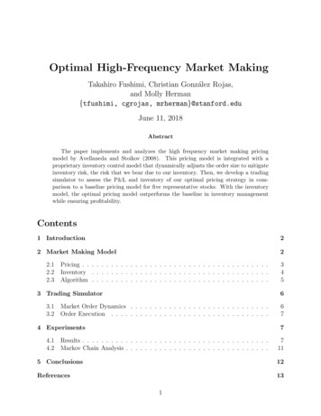
Then, this nonlinear partial differential equation is solved using an asymptotic expansion fora small inventory q. This results in the pricing equations that are relevant to our algorithm:(r(s, t) s qγσ 2 (T t) Indifference price δ a δ b γσ 2 (T t) ln 1 κγ Spread around r(s, t)It is important to notice that, since Avellaneda and Stoikov (2008) defines T as the terminaltime in which the trader optimizes its expected utility, the spread equation can be seen as alinear function of (T t) given by: γ ab2δ δ γσ (T t) ln 1 {z} {z κ }ABwhere A is the slope of the spread equationB is the closing spread when t TIf γ 0, the spread equation becomes a decreasing function of time. The rationale behind thisoptimal strategy is that tighter optimal spread enables the market marker to liquidate theirposition before the market closes so as to avoid overnight risk. To implement the frameworkdeveloped by Avellaneda and Stoikov (2008) we must compute our indifference price and setan optimal spread around it given by these two equations. We exploit the linearity of thespread equation and our market data in order to adjust our spread to the best bid-ask spreaddynamics. The calibration strategy is explained in detail in the Experiments section of thepaper.2.2InventoryTo complement the pricing model, we develop a proprietary dynamic order size framework.Unlike the strategy followed by Guéant et al. (2013), who stops quoting if the inventoryreaches the maximum permissible level, we are able to keep trading and earning rebates byadjusting the order size based on our current position. Our order size model is given by thefollowing equation:((maxφifq 0φmaxif qt 0tttaskφbid φ ttmax ηqtmax ηqtφt · eif qt 0φt · eif qt 0askwhere φbidare the bid and ask order size at time tt , φtmaxφtis the maximum order size at time tη is a shape parameterWe select the shape parameter η 0.005 to obtain dynamic order size model shown inFigure 1. As we will later see, this function is very effective at controlling inventory risk.The main reasoning behind its mechanics is that the framework controls inventory risk byplacing smaller order sizes in the direction of excess position accumulation.4

1008060Sell 100 sharesBuy at function2040Order SizeBuy 100 sharesSell at function-600-400-2000200400600PositionFigure 1: Dynamic order size function2.3AlgorithmAs a market maker, we are interested in implementing an algorithm that places bid and askquotes in the limit order book at all times. However, we are aware that in very brief periods,we must hold one-sided quotes for the sake of profitability. This situation occurs when bothbuy and sell orders are not filled at the same time interval.Therefore, our strategy iterates as follows. During the trading day, we quote a bid and askspread if we have no orders in the limit order book. If only one of these orders is filled, wewait for 5 seconds for the outstanding order to be executed. If this does not happen, thenwe cancel the order and place new bid and ask quotes. Finally, whenever we have two ordersin the limit order book, we update our quotes every second. The summary of the tradingalgorithm is shown in Algorithm 1.Algorithm 1 Market Making Algorithmwhile current time end time doif no orders in the book thenQuote bid and ask priceselse if 1 order in the book thenif current time - execution time waiting time thenCancel the outstanding order Quote new bid and ask priceselseWaitendelse if 2 orders in the book thenif current time - quote time update time thenCancel both order Quote new bid and ask priceselseWaitendendend5

3Trading SimulatorWe build a trading simulator to assess our strategy. The principal constituent of the simulatoris market order dynamics because as a market maker, we only use limit orders which arematched and filled by market orders. Given this model, we can simulate order executionsand run our market making strategy. For simplicity, we make the following assumptions: 1)No latency, 2) No price impact, and 3) No competition with other market makers.3.1Market Order DynamicsLet ξ denote the depth of our quote in the order book. We use a Time-InhomogeneousPoisson Process to model the number of arrivals of market orders that are matched with thelimit order at the depth of ξ: Z t Nt P oisλ(s, ξ)ds0Analogous to the market making model, the intensity function is assumed to be a productof time and depth components in the following form:λ(t, ξ) αt e µξA piece-wise linear bathtub shape is adopted for the time component αt based on the empiricalresult of intraday volume pattern as discussed in Cartea, Jaimungal, and Penalva (2015). Thedepth component e µξ is a decreasing function of depth ξ since the deeper a quote is, theless likely it is for the order to be executed due to the lower priority. Figure 3 illustrates theshape of these two components respectively.(a)(b)Time component αtDepth component e µξFigure 2: The shape of intensity function6