WIXLIB

1/8Optimal Chilled Water Delta-TTechnical Assistance to Flow Control Industries (FCI)Peter Armstrong and Dave Winiarski30 September 2006PNNL-16161PNNL OSBP Technical Assistance ProgramFCI markets a pressure-independent flow control valve for application at chilled water coils inair handlers served by a chilled water loop. Proper control of chilled water to the air handlersaffects the staging of upstream pumps and chillers. A common symptom of pump controlsequence error is low chilled water temperature difference (Delta-T) at part load. In thisscenario, the flow rate and head remain high even when the cooling load is a fraction of designload. Because flow rate and delta-T are inversely related, we can use the concepts of pumpsequencing, multi-speed control, and variable-speed control more or less interchangeably.The objective of this Technical Assistance project is a set of analysis tools to help design andoperating engineers determine the best control sequence for pumps and fans and to estimate theoperating cost penalty for improper chilled water pump sequencing manifest as low Delta-T.Delta-T is a shorthand term used in the HVAC industry for the chilled water temperature dropacross the evaporator, a function of cooling load and chilled-water flow rate.A Chiller Plant Control Tool is needed to generate the control sequences and setpoints or resetschedules that prevent excessive chiller compressor power on the one hand, and excessive fanand pump power on the other. Under a given set of conditions (outdoor temperature and returnair or return chilled water temperature) a given cooling load will be met with minimum totalpower when the relations between chiller, pump and fan power are properly balanced.In addition to determining the best control strategy for efficient operation of a HVAC plant, thedesigner should be able to estimate annual energy use and savings with respect to a faulty controlsequence. An Annual-Cost Estimating Tool is needed to estimate building loads and chiller plantperformance for a given control strategy.It is desirable to structure these tools so that actual characteristics of existing equipment andobserved building load information can be plugged in to ensure that the resulting analysis appliesto the plant in question—i.e. has specific relevance to the building owner or bill-paying tenants,and is not just a hypothetical paper study.In this report, preliminary designs of the chiller plant control tool and annual operating cost toolare presented. These preliminary designs illustrate the functions as well as the required inputdata. However, the component models used at this stage are simplified and the results presentedfor a simple test case are based on hypothetical plant parameters. Refinement of the models andrealistic test cases will be incorporated in the next phase of technical assistance.Chiller Plant Control ToolA prototype tool that may be used to find optimal speeds of the compressor, chilled water pumpand condenser fan has been developed. Although the use of a single compressor, single pumpand single fan is the simplest of possible topologies, it does illustrate the sensitivity of plantperformance to delta-T as pump speed is varied. This tool can be readily extended to model awide variety of plants with multiple chillers and multiple fans and pumps on the condenser andevaporator sides of the compressors.

2/8The plant parameters for an air-cooled chiller must be specified as follows.Chiller performance maps:Qcmpr (kBtu/h) fc(ρs, Ps, Pd, Sc) andEcmpr (kW) fp(ρs, Ps, Pd, Sc) whereρs suction density,Ps, Pd suction and discharge pressures, andSc compressor shaft speed.Evaporator pump and heat exchanger parameters:Ceo (kBtu/h/F) evaporator chilled water design thermal capacitance rate,Eeo (kW) pump power at design thermal capacitance rate, andUAeo (kBtu/h/F) evaporator heat exchanger conductance.Condenser fan and heat exchanger parameters:Cco (kBtu/h/F) condenser fan design thermal capacitance rate,Eco (kW) fan power at design thermal capacitance rate, andUAco (kBtu/h/F) condenser heat exchanger conductance.In addition, the conditions and cooling load are specified:TODB outdoor temperatureTr chilled water return temperatureQ total chilled water cooling load.The combination of pump, fan and compressor speed that satisfies load with the least total plantpower are solved for using the relationships developed in Appendix A. A typical solution isshown in Table 1.Table 1. Motor speed solution for one set of boundary conditions (BC).Solution: Te,TcFBC:Tr,TODBFBC: cooling load, QkBtu/hPump/fan parameters: Eeo, EcokWHX Parameters: Ceo, CcokBtu/h/FHX Parameters: UAe, UAckBtu/h/FQ/dt (input to HX solver)kBtu/h/FHX solutions Ce, CckBtu/h/F3Suction density, ρLbm/ftSuction Pe, Discharge PcpsiaRefrig’t vapor enthalpies he,hcBtu/lbmCompressor speed Sc/SoCompressor capacity (Btuh), power (kW)Pump, fan power Ee,EckWJ Ee Ec 3025815Solutions for a range of loads and conditions are presented in Figure 1. The response surfacesrepresented in Figure 1 can be evaluated from tabular data (Appendix B) by linear interpolation.The following trends are noted.Efficiency. With optimal control of fan, pump and compressor, the overall plant efficiency,EER (cooling effect kBtuh)/(total kW), increases as load decreases. This is primarily the resultof reduced flow losses (fan and pump power decrease faster than cooling load) and closerapproach temperatures (compressor power decreases slightly faster than load).

3/8408357306255204153EER (Btu/Wh)delta-Tcompressor powertotal power (kW)105Input Power (kW)EER (Btu/Wh), delta-T (F)nf\smprj\FCI2\compr3.xls P Q,T21001020304050Qload (kBtuh)607080900100Figure 1. Solutions for range of cooling loads and TODB 60:10:100 F. Within each family ofcurves, power and delta-T increase while EER decreases with TODB.Plant Electrical Load. Total plant power is almost linear with load because, under optimalcontrol, it is dominated by compressor power--even at the lightest of partial cooling loads.Delta-T. Chilled water temperature delta-T is relatively constant under optimal control of fan,pump and compressor. There is only a 17% reduction from design delta-T at the 50% part-loadmark.Annual Cost ToolA bin method used to estimate annual operating cost of package equipment (www.pnl.gov/uac)has been adapted to estimate chiller plant operating costs.To estimate seasonal performance we must specify, in addition to chiller plant performance, aclimate and a load. We must also specify energy prices.A spreadsheet version of the UAC calculator is shown in Table 2. The load model assumes asensible cooling load directly proportional to outdoor temperature and a latent load directlyproportional to the product of outdoor humidity (mass ratio of water vapor to dry air) and outsideair flow rate. An ideal enthalpy control is assumed and a fixed minimum outside air flow rate(10% in this analysis) is specified by the user. The peak load (for sizing purposes) is assumed tooccur at the ASHRAE 0.4% dry- and coincident wet-bulb temperatures with the minimum (40scfm/Ton) 1 outside air-flow setting.The cooling balance point must also be specified. Here balance point is defined as the thermostat setpoint minus the ratio of average solar and internal gains 2 to envelope UA. For example,with a 75 F setpoint, average gains of 150 kBtu/h and a UA of 60 kBtu/h/ F, the balance point is75 – 150/60 50 F.1240 scfm per Ton of cooling capacity corresponds to about 10% outside air, a typical minimum outside air fractionAverage over occupied hours, including metabolic heat output of occupants.

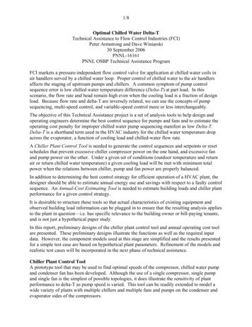
4/8Table 2. Chiller Plant Operation Cost Calculator.CHILLER PLANT ANNUAL ENERGY, DEMAND, AND COST CALCULATIONLocation:Atlanta, GABalance PointEconomizerConstant-speed fans & pumpsGHIJKLMNDemand ChargesEnergy Charges0Plant kW, (f(I,A,B))Ratchet ( /kW)Remaining Load AfterEconomizerF FEconomizer CoolingCapacity kBtu/hSeasonal Cooling Hours,TMYE00Total Heat Gain, kBtu/h(E F)DNumber of Months withthis Peak hour, TMYCOutdoor TemperatureDifference (A–Tbalance)Outdoor Temperature 5 FIncrementsCooling LoadBCoincident Wet BulbTemperature, FWeather ConditionsA52Winter demand ( /kW)Ventilation Heat Gain,kBtu/h FSummer demand ( /kW)Sensible Heat 558.80224Sequenced fans & pumpsOPQEnergy ChargesWet Bulb:115Demand ChargesDesign LoadVentilation CFMPlant kW, (f(I,A,B))Electric rate ( /kWh)ASHRAE 0.4% Design ConditionsDry Bulb:93 .009.827.6710.009.821000 0.00 1,624.95 0.00 1,183.660105110115Total Annual CostsOutdoor temperature bins represent the median temperature (i.e. 60 F is the range of temperatures between 57.5 F through 62.5 F)

5/8The hourly coil load is evaluated by the load model for a given bin temperature The chiller plantmodel is then applied to determine average kW for the bin and this is multiplied by the number ofannual bin hours to get bin kWh. The resulting kWh numbers are then summed over all bins toget the annual operating energy. The bin energy charge is the product of bin kWh and price. Fortime-of-use rates one must use a blended rate in which the summer on-peak rate is given extraweight appropriate for the seasonal and time-of-day distribution of chiller plant electrical use.The monthly peak demands can be estimated from the bins corresponding to the 12 monthly peakcooling load conditions. The bin demand charge is the product of bin demand, its correspondingnumber of months, and the demand charge. The numbers of months may be decomposed intoseparate summer and winter columns to allow for different summer and winter demand rates.Annual energy and demand charges are summed and appear at the foot of each column.Conclusions and RecommendationsThis report contains the preliminary draft versions of a chiller plant control sequence tool and anannual operating cost tool. Following a review of this report by FCI, further refinement of thecomponent models used in the tools and more realistic test cases will be added in the next phase ofthe technical assistance project.BibliographyArmstrong, PR, DW Winiarski, and S Somasundaram, 2004. Preliminary Analysis of PressureIndependent Flow Control for Cooling Coils, TGA PNNL-14417Bahnfleth, William P. and Eric B. Peyer, 2004, Varying views on variable-primary flow: chilledwater systems, HPAC, March.Bahnfleth, William P. and Eric B. Peyer, 2001, Comparative analysis of chilled-water-plantperformance, HPAC, April.Bellenger, Lynn G., 2003, Revisiting chiller retrofits to replace constant volume pumps, HPAC,September.Braun J E., Klein S A., Beckman W A., Mitchell J W. 1989. Methodologies for optimal control ofchilled water systems without storage, ASHRAE Trans. 95(1): 652-662.Braun J E., Klein S A., Mitchell J W., Beckman W A. 1989. Applications of optimal control tochilled water systems without storage, ASHRAE Trans. 95(1): 663-675.Braun, J, SA Klein and JW Mitchell. 1989. Effectiveness models for cooling towers and coolingcoils. ASHRAE Trans. 95(2): 164-174.Braun J E., Diderrich G T. 1990. Near-optimal control of cooling towers for chilled water systems,ASHRAE Trans. 96(2): 806-813.Coad, WJ, 1985. Variable flow in hydronic systems for improved stability, simplicity and energyeconomics, ASHRAE Transactions, 91(1) 224-237.Ding, X, JP Eppe, J Lebrun, M Wasacz. 1990. Cooling coil model to be used in transient and/orwet regimes: theoretical analysis and experimental validation. Proc. Third IBPSA Conf., Liege.405-441.Elmahdy, AH and GP Mitalas. 1977. A simple model for cooling and dehumidifying coils for usein calculating energy requirements in buildings. ASHRAE Trans. 83(2): 103-117.