Transcription
SparkThe Definitive GuideExcerpts from the upcoming book on makingbig data simple with Apache Spark.By Bill Chambers & Matei Zaharia1
PrefaceApache Spark has seen immense growth over the pastseveral years. The size and scale of Spark Summit 2017 isa true reflection of innovation after innovation that hasmade itself into the Apache Spark project. Databricksis proud to share excerpts from the upcoming book,Spark: The Definitive Guide. Enjoy this free preview copy,courtesy of Databricks, of chapters 2, 3, 4, and 5 andsubscribe to the Databricks blog for upcoming chapterreleases.2
A Gentle Introduction to SparkThis chapter will present a gentle introduction to Spark. We will walk through the core architecture of a cluster, SparkApplication, and Spark’s Structured APIs using DataFrames and SQL. Along the way we will touch on Spark’s coreterminology and concepts so that you are empowered start using Spark right away. Let’s get started with some basicbackground terminology and concepts.Spark’s Basic ArchitectureTypically when you think of a “computer” you think about one machine sitting on your desk at home or at work. Thismachine works perfectly well for watching movies or working with spreadsheet software. However, as many userslikely experience at some point, there are some things that your computer is not powerful enough to perform. Oneparticularly challenging area is data processing. Single machines do not have enough power and resources to performcomputations on huge amounts of information (or the user may not have time to wait for the computation to finish).A cluster, or group of machines, pools the resources of many machines together allowing us to use all the cumulativeresources as if they were one. Now a group of machines alone is not powerful, you need a framework to coordinatework across them. Spark is a tool for just that, managing and coordinating the execution of tasks on data across acluster of computers.The cluster of machines that Spark will leverage to execute tasks will be managed by a cluster manager like Spark’sStandalone cluster manager, YARN, or Mesos. We then submit Spark Applications to these cluster managers which willgrant resources to our application so that we can complete our work.Spark ApplicationsSpark Applications consist of a driver process and a set of executor processes. The driver process, Figure 1-2, sitson a node in the cluster and is responsible for three things: maintaining information about the Spark application;responding to a user’s program; and analyzing, distributing, and scheduling work across the executors. As suggestedby the following figure, the driver process is absolutely essential - it’s the heart of a Spark Application and maintainsall relevant information during the lifetime of the application.3
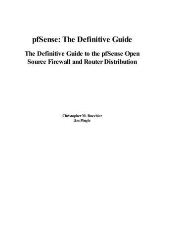
Spark ApplicationJVMSpark SessionTo ExecutorsUser CodeFigureThe driver maintains the work to be done, the executors are responsible for only two things: executing code assignedto it by the driver and reporting the state of the computation, on that executor, back to the driver node.The last piece relevant piece for us is the cluster manager. The cluster manager controls physical machines andallocates resources to Spark applications. This can be one of several core cluster managers: Spark’s standalonecluster manager, YARN, or Mesos. This means that there can be multiple Spark applications running on a cluster atthe same time. We will talk more in depth about cluster managers in Part IV: Production Applications of this book. Inthe previous illustration we see on the left, our driver and on the right the four executors on the right. In this diagram,we removed the concept of cluster nodes. The user can specify how many executors should fall on each node throughconfigurations.noteSpark, in addition to its cluster mode, also has a local mode. The driver and executors are simply processes, thismeans that they can live on a single machine or multiple machines. In local mode, these run (as threads) on yourindividual computer instead of a cluster. We wrote this book with local mode in mind, so everything should berunnable on a single machine.As a short review of Spark Applications, the key points to understand at this point are that: Spark has some cluster manager that maintains an understanding of the resources available. The driver process is responsible for executing our driver program’s commands accross the executors in order tocomplete our task.Now while our executors, for the most part, will always be running Spark code. Our driver can be “driven” from anumber of different languages through Spark’s Language APIs.4
Driver ProcessExecutorsSpark SessionUser CodeCluster ManagerFigure 2:Spark’s Language APIsSpark’s language APIs allow you to run Spark code from other langauges. For the most part, Spark presents some core“concepts” in every language and these concepts are translated into Spark code that runs on the cluster of machines.If you use the Structured APIs (Part II of this book), you can expect all languages to have the same performancecharacteristics.noteThis is a bit more nuanced than we are letting on at this point but for now, it’s true “enough”. We cover thisextensively in first chapters of Part II of this book.5
ScalaSpark is primarily written in Scala, making it Spark’s “default” language. This book will include Scala code exampleswherever relevant.PythonPython supports nearly all constructs that Scala supports. This book will include Python code examples whenever weinclude Scala code examples and a Python API exists.SQLSpark supports ANSI SQL 2003 standard. This makes it easy for analysts and non-programmers to leverage the bigdata powers of Spark. This book will include SQL code examples wherever relevantJavaEven though Spark is written in Scala, Spark’s authors have been careful to ensure that you can write Spark code inJava. This book will focus primarily on Scala but will provide Java examples where relevant.RSpark has two libraries, one as a part of Spark core (SparkR) and another as a R community driven package (sparklyr).We will cover these two different integrations in Part VII: Ecosystem.6
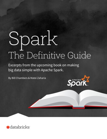
JVMPython/R ProcessSpark SessionUser CodeFigureHere’s a simple illustration of this relationship.Each language API will maintain the same core concepts that we described above. There is a SparkSession availableto the user, the SparkSession will be the entrance point to running Spark code. When using Spark from a Python orR, the user never writes explicit JVM instructions, but instead writes Python and R code that Spark will translate intocode that Spark can then run on the executor JVMs. There is plenty more detail about this implementation that wecover in later parts of the book but for the most part the above section should be plenty for you to use and leverageSpark successfully.Starting SparkThus far we covered the basics concepts of Spark Applications. At this point it’s time to dive into Spark itself andunderstand how we actually go about leveraging Spark. To do this we will start Spark’s local mode, just like we didin the previous chapter, this means running ./bin/spark-shell to access the Scala console. You can also startPython console with ./bin/pyspark. This starts an interactive Spark Application. There is another method forsubmitting applications to Spark called spark-submit which does not allow for a user console but instead executesprepared user code on the cluster as its own application. We discuss spark-submit in Part IV of the book. When westart Spark in this interactive mode, we implicitly create a SparkSession which manages the Spark Application.SparkSessionAs discussed in the beginning of this chapter, we control our Spark Application through a driver process. This driverprocess manifests itself to the user as something called the SparkSession. The SparkSession instance is the way Sparkexeutes user-defined manipulations across the cluster. In Scala and Python the variable is available as spark whenyou start up the console. Let’s go ahead and look at the SparkSession in both Scala and/or Python.7
sparkIn Scala, you should see something like:res0: org.apache.spark.sql.SparkSession org.apache.spark.sql.SparkSession@27159a24In Python you’ll see something like: pyspark.sql.session.SparkSession at 0x7efda4c1ccd0 Let’s now perform the simple task of creating a range of numbers. This range of numbers is just like a named columnin a spreadsheet.%scalaval myRange spark.range(1000).toDF(“number”)%pythonmyRange spark.range(1000).toDF(“number”)You just ran your first Spark code! We created a DataFrame with one column containing 1000 rows with values from0 to 999. This range of number represents a distributed collection. When run on a cluster, each part of this range ofnumbers exists on a different executor. This range is what Spark defines as a DataFrame.DataFramesA DataFrame is a table of data with rows and columns. The list of columns and the types in those columns is theschema. A simple analogy would be a spreadsheet with named columns. The fundamental difference is that while aspreadsheet sits on one computer in one specific location, a Spark DataFrame can span thousands of computers. Thereason for putting the data on more than one computer should be intuitive: either the data is too large to fit on onemachine or it would simply take too long to perform that computation on one machine. The DataFrame concept is notunique to Spark. R and Python both have similar concepts. However, Python/R DataFrames (with some exceptions)exist on one machine rather than multiple machines. This limits what you can do with a given DataFrame in pythonand R to the resources that exist on that specific machine. However, since Spark has language interfaces for bothPython and R, it’s quite easy to convert to Pandas (Python) DataFrames8
Spreadsheet on asingle machineTable or DataFrame partitionedacross servers in data centerFigurenoteSpark has several core abstractions: Datasets, DataFrames, SQL Tables, and Resilient Distributed Datasets(RDDs). These abstractions all represent distributed collections of data however they have different interfacesfor working with that data. The easiest and most efficient are DataFrames, which are available in all languages.We cover Datasets at the end of Part II and RDDs in Part III of this book. The following concepts apply to all of thecore abstractions.PartitionsIn order to allow every executor to perform work in parallel, Spark breaks up the data into chunks, called partitions. Apartition is a collection of rows that sit on one physical machine in our cluster. A DataFrame’s partitions represent howthe data is physically distributed across your cluster of machines during execution. If you have one partition, Sparkwill only have a parallelism of one even if you have thousands of executors. If you have many partitions, but only oneexecutor Spark will still only have a parallelism of one because there is only one computation resource.An important thing to note, is that with DataFrames, we do not (for the most part) manipulate partitions individually.We simply specify high level transformations of data in the physical partitions and Spark determines how this workwill actually execute on the cluster. Lower level APIs do exist (via the RDD interface) and we cover those in Part III ofthis book.TransformationsIn Spark, the core data structures are immutable meaning they cannot be changed once created. This might seem likea strange concept at first, if you cannot change it, how are you supposed to use it? In order to “change” a DataFrameyou will have to instruct Spark how you would like to modify the DataFrame you have into the one that you want.These instructions are called transformations.9
Let’s perform a simple transformation to find all even numbers in our currentDataFrame.%scalaval divisBy2 myRange.where(“number % 2 0”)%pythondivisBy2 myRange.where(“number % 2 0”)You will notice that these return no output, that’s because we only specified an abstract transformation and Sparkwill not act on transformations until we call an action, discussed shortly. Transformations are the core of how youwill be expressing your business logic using Spark. There are two types of transformations, those that specify narrowdependencies and those that specify wide dependencies. Transformations consisting of narrow dependenciesare those where each input partition will contribute to only one output partition. Our where clause specifies anarrow dependency, where only one partition contributes to at most one output partition. A wide dependency styletransformation will have input partitions contributing to many output partitions. We call this a shuffle where Sparkwill exchange partitions across the cluster. Spark will automatically perform an operation called pipelining on narrowdependencies, this means that if we specify multiple filters on DataFrames they’ll all be performed in memory. Thesame cannot be said for shuffles. When we perform a shuffle, Spark will write the results to disk. You’ll see lots of talksabout shuffle optimization across the web because it’s an important topic but for now all you need to understand arethat there are two kinds of transformations.This brings ups our next concept, transformations are abstract manipulations of data that Spark will execute lazily.Lazy EvaluationLazy evaulation means that Spark will wait until the very last moment to execute your transformations. In Spark,instead of modifying the data quickly, we build up a plan of transformations that we would like to apply to our sourcedata. Spark, by waiting until the last minute to execute the code, will compile this plan from your raw, DataFrametransformations, to an efficient physical plan that will run as efficiently as possible across the cluster. This providesimmense benefits to the end user because Spark can optimize the entire data flow from end to end. An example of thismight be “predicate pushdown”. If we build a large Spark job consisting of narrow dependencies, but specify a filter atthe end that only requires us to fetch one row from our source data, the most efficient way to execute this is to accessthe single record that we need. Spark will actually optimize this for us by pushing the filter down automatically.10
ActionsTransformations allow us to build up our logical transformation plan. To trigger the computation, we run an action. Anaction instructs Spark to compute a result from a series of transformations. The simplest action is count which givesus the total number of records in the DataFrame.divisBy2.count()We now see a result! There are 500 number divisible by two from o to 999 (big surprise!). Now count is not the onlyaction. There are three kinds of actions: actions to view data in the console; actions to collect data to native objects in the respective language; and actions to write to output data sources.In specifying our action, we started a Spark job that runs our filter transformation (a narrow transformation), then anaggregation (a wide transformation) that performs the counts on a per partition basis, then a collect will brings ourresult to a native object in the respective language. We can see all of this by inspecting the Spark UI, a tool included inSpark that allows us to monitor the Spark jobs running on a cluster.Spark UIDuring Spark’s execution of the previous code block, users can monitor the progress of their job through the Spark UI.The Spark UI is available on port 4040 of the driver node. If you are running in local mode this will just be thehttp://localhost:4040. The Spark UI maintains information on the state of our Spark jobs, environment, andcluster state. It’s very useful, especially for tuning and debugging. In this case, we can see one Spark job with twostages and nine tasks were executed.This chapter avoids the details of Spark jobs and the Spark UI. At this point you should understand that a Spark jobrepresents a set of transformations triggered by an individual action and we can monitor that from the Spark UI. Wedo cover the Spark UI in detail in Part IV: Production Applications of this book.11
Figure 5An End to End ExampleIn the previous example, we created a DataFrame of a range of numbers. Not exactly groundbreaking big data. Inthis section we will reinforce everything we learned previously in this chapter with a worked example and explainingstep by step what is happening under the hood. We’ll be using some flight data available here from the United StatesBureau of Transportation statistics.Inside of the CSV folder linked above, you’ll see that we have a number of files. You will also notice a number of otherfolders with different file formats that we will discuss in Part II: Reading and Writing data.%fs ls /mnt/defg/flight-data/csv/Each file has a number of rows inside of it. Now these files are CSV files, meaning that they’re a semi-structured dataformat with a row in the file representing a row in our future DataFrame. head /mnt/defg/flight-data/csv/2015-summary.csvDEST COUNTRY NAME,ORIGIN COUNTRY NAME,countUnited States,Romania,15United States,Croatia,1United States,Ireland,34412
Spark includes the ability to read and write from a large number of data sources. In order to read this data in, we willuse a DataFrameReader that is associated with our SparkSession. In doing so, we will specify the file format as well asany options we want to specify. In our case, we want to do something called schema inference, we want Spark to takea best guess at what the schema of our DataFrame should be. The reason for this is that CSV files are not completelystructured data formats. We also want to specify that the first row is the header in the file, we’ll specify that as anoption too.To get this information Spark will read in a little bit of the data and then attempt to parse the types in those rowsaccording to the types available in Spark. You’ll see that it does a good job. We also have the option of strictlyspecifying a schema when we read in data.%scalaval flightData2015 spark.read.option(“inferSchema”, “true”).option(“header”, summary.csv”)%pythonflightData2015 spark\.read\.option(“inferSchema”, “true”)\.option(“header”, -summary.csv”)Each of these DataFrames (in Scala and Python) each have a set of columns with an unspecified number of rows.The reason the number of rows is “unspecified” is because reading data is a transformation, and is therefore a lazyoperation. Spark only peeked at the data to try to guess what types each column should be.JSONfileflightData2015DataFramereadtake (2)LazyEagerArray( Row(.),Row(.))Figure13
If we perform the take action on the DataFrame, we will be able to see the same results that we saw before when weused the command line.flightData2015.take(3)Let’s specify some more transformations! Now we will sort our data according to the count column which is aninteger type.noteRemember, the sort does not modify the DataFrame. We use the sort is a transformation that returns a newDataFrame by transforming the previous DataFrame. Let’s take a look at this transformation as an illustration.JSON fileDataFrameReadDataFrameSortFigure 7:Nothing will happen to the data when we call this sort because it’s just a transformation. However, we can see thatSpark is building up a plan for how it will execute this across the cluster by looking at the explain plan. We can callexplain on any DataFrame object to see the DataFrame’s Congratulations, you’ve just read your first explain plan! Explain plans are a bit arcane, but with a bit of practice itbecomes second nature. Explain plans can be read from top to bottom, the top being the end result and the bottom14
being the source(s) of data. In our case, just take a look at the first keywords. You will see “sort”, “exchange”, and“FileScan”. That’s because the sort of our data is actually a wide dependency because rows will have to be comparedwith one another. Don’t worry too much about understanding everything about explain plans, they can just be helpfultools for debugging and improving your knowledge as you progress with Spark.Now, just like we did before, we can specify an action in order to kick off this plan.flightData2015.sort(“count”).take(2)This will get us the sorted results, as expected. This operation is illustrated in the following image.The logical plan of transformations that we build up defines a lineage for the DataFrame so that at any given point intime Spark knows how to recompute any partition by performing all of the operations it had before on the same inputdata. This sits at the heart of Spark’s programming model, functional programming where the same inputs alwaysresult in the same outputs when the transformations on that data stay constant.JSON eNow that we performed this action, remember that we can navigate to the Spark UI (port 4040) and see theinformation about this jobs stages and tasks.DataFrames and SQLWe worked through a simple example in the previous example, let’s now work through a more complex example andfollow along in both DataFrames and SQL. For your purposes, DataFrames and SQL, in Spark, are the exact samething. You can express your business logic in either language and Spark will compile that logic down to an underlyingplan (that we see in the explain plan) before actually executing your code. Spark SQL allows you as a user to registerany DataFrame as a table or view (a temporary table) and query it using pure SQL. There is no performance differencebetween writing SQL queries or writing DataFrame code, they both “compile” to the same underlying plan that wespecify in DataFrame code.15
Any DataFrame can be made into a table or view with one simple method “flight data iew(“flight data 2015”)Now we can query our data in SQL. To execute a SQL query, we’ll use the spark.sql function (remember spark isour SparkSession variable?) that conveniently, returns a new DataFrame. While this may seem a bit circular in logic- that a SQL query against a DataFrame returns another DataFrame, it’s actually quite powerful. As a user, you canspecify transformations in the manner most convenient to you at any given point in time and not have to trade anyefficiency to do so! To understand that this is happening, let’s take a look at two explain plans.%scalaval sqlWay spark.sql(“””SELECT DEST COUNTRY NAME, count(1)FROM flight data 2015GROUP BY DEST COUNTRY NAME“””)val dataFrameWay flightData2015.groupBy(‘DEST COUNTRY thonsqlWay spark.sql(“””SELECT DEST COUNTRY NAME, count(1)FROM flight data 2015GROUP BY DEST COUNTRY NAME“””)16
dataFrameWay flightData2015\.groupBy(“DEST COUNTRY ain()We can see that these plans compile to the exact same underlying plan!To reinforce the tools available to us, let’s pull out some interesting statistics from our data. One thing to understandis that DataFrames (and SQL) in Spark already have a huge number of manipulations available. There are hundredsof functions that you can leverage and import to help you resolve your big data problems faster. We will use the maxfunction, to find out what the maximum number of flights to and from any given location are. This just scans eachvalue in relevant column the DataFrame and sees if it’s bigger than the previous values that have been seen. This is atransformation, as we are effectively filtering down to one row. Let’s see what that looks like.// scala or pythonspark.sql(“SELECT max(count) from flight data 2015”).take(1)%scalaimport elect(max(“count”)).take(1)%pythonfrom pyspark.sql.functions import Great, that’s a simple example. Let’s perform something a bit more complicated and find out the top five destinationcountries in the data set? This is a our first multi-transformation query so we’ll take it step by step. We will start with afairly straightforward SQL aggregation.17
%scalaval maxSql spark.sql(“””SELECT DEST COUNTRY NAME, sum(count) as destination totalFROM flight data 2015GROUP BY DEST COUNTRY NAMEORDER BY sum(count) DESCLIMIT 5“””)maxSql.collect()%pythonmaxSql spark.sql(“””SELECT DEST COUNTRY NAME, sum(count) as destination totalFROM flight data 2015GROUP BY DEST COUNTRY NAMEORDER BY sum(count) DESCLIMIT 5“””)maxSql.collect()Now let’s move to the DataFrame syntax that is semantically similar but slightly different in implementation andordering. But, as we mentioned, the underlying plans for both of them are the same. Let’s execute the queries and seetheir results as a sanity check.%scalaimport groupBy(“DEST COUNTRY (count)”, “destination total”).sort(desc(“destination total”)).limit(5).collect()18
%pythonfrom pyspark.sql.functions import descflightData2015\.groupBy(“DEST COUNTRY um(count)”, “destination total”)\.sort(desc(“destination total”))\.limit(5)\.collect()Now there are 7 steps that take us all the way back to the source data. You can see this in the explain plan on thoseDataFrames. Illustrated below are the set of steps that we perform in “code”. The true execution plan (the one visiblein explain) will differ from what we have below because of optimizations in physical execution, however the llustrationis as good of a starting point as any. This execution plan is a directed acyclic graph (DAG) of transformations, eachresulting in a new immutable DataFrame, on which we call an action to generate a result.CSV fileDataFrameReadGrouped DatasetgroupByDataFrameArray(.)Our nrenamedSortFigure 9:The first step is to read in the data. We defined the DataFrame previously but, as a reminder, Spark does not actuallyread it in until an action is called on that DataFrame or one derived from the original DataFrame.The second step is our grouping, technically when we call groupBy we end up with a RelationalGroupedDatasetwhich is a fancy name for a DataFrame that has a grouping specified but needs a user to specify an aggregation beforeit can be queried further. We can see this by trying to perform an action on it (which will not work). We still haven’tperformed any computation (besides relational algebra) - we’re simply passing along information about the layout of19
the data.Therefore the third step is to specify the aggregation. Let’s use the sum aggregation method. This takes as inputa column expression or simply, a column name. The result of the sum method call is a new dataFrame. You’ll seethat it has a new schema but that it does know the type of each column. It’s important to reinforce (again!) that nocomputation has been performed. This is simply another transformation that we’ve expressed and Spark is simplyable to trace the type information we have supplied.The fourth step is a simple renaming, we use the withColumnRenamed method that takes two arguments, theoriginal column name and the new column name. Of course, this doesn’t perform computation - this is just anothertransformation!The fifth step sorts the data such that if we were to take results off of the top of the DataFrame, they would be thelargest values found in the destination total column.You likely noticed that we had to import a function to do this, the desc function. You might also notice that descdoes not return a string but a Column. In general, many DataFrame methods will accept Strings (as column names) orColumn types or expressions. Columns and expressions are actually the exact same thing.The final step is just a limit. This just specifies that we only want five values. This is just like a filter except that it filtersby position (lazily) instead of by value. It’s safe to say that it basically just specifies a DataFrame of a certain size.The last step is our action! Now we actually begin the process of collecting the results of our DataFrame above andSpark will give us back a list or array in the language that we’re executing. Now to reinforce all of this, let’s look at theexplain plan for the above query.%scalaflightData2015.groupBy(“DEST COUNTRY (count)”, “destination total”).sort(desc(“destination \.groupBy(“DEST COUNTRY um(count)”, “destination total”)\20
.sort(desc(“destination total”))\.limit(5)\.explain() Physical Plan TakeOrderedAndProject(limit 5, orderBy [destination total#16194L DESC],output [DEST COUNTRY - *HashAggregate(keys [DEST COUNTRY NAME#7323], functions [sum(count#7325L)]) - Exchange hashpartitioning(DEST COUNTRY NAME#7323, 5) - *HashAggregate(keys [DEST COUNTRY NAME#7323], functions [partialsum(count#7325L)]) - InMemoryTableScan [DEST COUNTRY NAME#7323, count#7325L] - InMemoryRelation [DEST COUNTRY NAME#7323, ORIGIN COUNTRY NAME#7324, count# - *Scan csv [DEST COUNTRY NAME#7578,ORIGIN COUNTRY NAME#7579,count#7580L]While this explain plan doesn’t match our exact “conceptual plan” all of the pieces are there. You can see the limitstatement as well as the orderBy (in the first line). You can also see how our aggregation happens in two phases, inthe partial sum calls. This is because summing a list of numbers is commutative and Spark can perform the sum,partition by partition. Of course we can see how we read in the DataFrame as well.Naturally, we don’t always have to collect the data. We can a
Apache Spark has seen immense growth over the past several years. The size and scale of Spark Summit 2017 is a true reflection of innovation after innovation that has made itself into the Apache Spark project. Databricks is proud to share excerpts from the upcoming book, Spark: The Definitive Guide. Enjoy this free preview copy,