Transcription
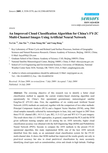
Sensors 2009, 9, 5558-5579; doi:10.3390/s90705558OPEN ACCESSsensorsISSN 1424-8220www.mdpi.com/journal/sensorsArticleAn Improved Cloud Classification Algorithm for China’s FY-2CMulti-Channel Images Using Artificial Neural NetworkYu Liu 1,2, Jun Xia 1,*, Chun-Xiang Shi 3 and Yang Hong 41234Key Laboratory of Water Cycle and Related Land Surface Processes, Institute of GeographicSciences and Natural Resources Research, Chinese Academy of Sciences, Beijing, 100101, China;E-Mail: liuyu950@126.comGraduate School of the Chinese Academy of Science, CAS, Beijing,100039, ChinaNational Satellite Meteorological Center, Beijing 100081, China; E-Mail: shicx@cma.gov.cmSchool of Civil Engineering and Environmental Sciences, University of Oklahoma, NationalWeather Center Suite 3630, Norman, OK 73019, USA; E-Mail: yanghong@ou.edu* Author to whom correspondence should be addressed; E-Mail: xiaj@igsnrr.ac.cn;Tel.: 86-10-64889312; Fax: 86-10-64856534Received: 16 June 2009; in revised form: 7 July 2009 / Accepted: 7 July 2009/Published: 14 July 2009Abstract: The crowning objective of this research was to identify a better cloudclassification method to upgrade the current window-based clustering algorithm usedoperationally for China’s first operational geostationary meteorological satelliteFengYun-2C (FY-2C) data. First, the capabilities of six widely-used Artificial NeuralNetwork (ANN) methods are analyzed, together with the comparison of two other methods:Principal Component Analysis (PCA) and a Support Vector Machine (SVM), using 2864cloud samples manually collected by meteorologists in June, July, and August in 2007 fromthree FY-2C channel (IR1, 10.3-11.3 μm; IR2, 11.5-12.5 μm and WV 6.3-7.6 μm) imagery.The result shows that: (1) ANN approaches, in general, outperformed the PCA and the SVMgiven sufficient training samples and (2) among the six ANN networks, higher cloudclassification accuracy was obtained with the Self-Organizing Map (SOM) and ProbabilisticNeural Network (PNN). Second, to compare the ANN methods to the present FY-2Coperational algorithm, this study implemented SOM, one of the best ANN networkidentified from this study, as an automated cloud classification system for the FY-2Cmulti-channel data. It shows that SOM method has improved the results greatly not only inpixel-level accuracy but also in cloud patch-level classification by more accuratelyidentifying cloud types such as cumulonimbus, cirrus and clouds in high latitude. Findings
Sensors 2009, 95559of this study suggest that the ANN-based classifiers, in particular the SOM, can bepotentially used as an improved Automated Cloud Classification Algorithm to upgrade thecurrent window-based clustering method for the FY-2C operational products.Keywords: FY-2C; multi-channel satellite image; ANN; cloud classification1. IntroductionClouds play an important role in the Earth system. They significantly affect the heat budget byreflecting short-wave radiation [1], and absorbing and emitting long-wave radiation [2]. The net effectis a function of the cloud optical properties and the properties of the underlying surface [3]. Differenttypes of clouds have different radiative effects on the Earth surface-atmosphere system. Accurate andautomatic cloud detection and classification are useful for numerous climatic, hydrologic andatmospheric applications [4]. Therefore, an accurate and cost-effective method of cloud detection andclassification based on satellite images has been a great interest of many scientists [5,6].Cloud classification methods can mainly be divided into following categories: the thresholdapproach, traditional statistical methods and new methods such as Artificial Neural Network (ANN).The threshold methods were mainly developed during the 1980s and early 1990s. They apply a set ofthresholds (both static and dynamic) of reflectance, brightness temperature and brightness temperaturedifference [7,8]. They are the simplest and probably most commonly used methods. However, thesemethods may fail when two different classes have no obvious brightness temperature difference (i.e.,indistinct threshold) because of the complexity of the cloud system. The traditional statistical methods,such as clustering method, histogram approach and others [9-11] are supposed to be superior to thethreshold methods to conduct cloud classification and detection in that they digest more information byusing all the available bands but they can hardly separate clusters with significant overlapping spaces.With a rapid development in technological innovations, at present, some new methods, such asneural network [12], Bayesian methods [13], maximum likelihood [14] and fuzzy logic [6], haveprovided impressive results for cloud detection and classification. Many studies have acknowledgedthat the well-trained cloud classification neural networks usually have relatively superiorperformance [15,16]. In fact, almost all the classification methods in the first two categories can be seenas a special or simpler case of neural networks [17]. Therefore, since the first application of ANN incloud classification [12], lots of ANN methods have been applied to satellite infrared images. Forexample MLP (Multilayer Perceptron) on LandSAT [18] and on NOAA-AVHRR [19], PNN(Probabilistic Neural Network) on GOES-8 and AVHRR [20,21], the combination of PNN and SOM(Self-Organizing Map) on Meteosat-7 [22], RBF (Radial Basis Functions) on GMS-5 [23,24] and soon. However, there is inadequate study to evaluate the performance and capacity of these ANNclassifiers on multi-channels satellite imagery. Historically, due to diversity of cloud dynamics andcomplexity of underlying surface, it is not uncommon to find out that single Infrared channel datacould not effectively identify cloud types because different cloud types might have similar cloud-topbrightness temperatures (Tbb).The intention of this study was to evaluate the performance of several widely used classificationalgorithms (ANN and statistical classifiers) on three data channels (IR1, 10.3-11.3 μm; IR2,
Sensors 2009, 9556011.5-12.5 μm and WV 6.3-7.6 μm) from China’s first operational geostationary meteorological satelliteFemgYu-2C (FY-2C). FY-2C was launched successfully from Xichang city, Sichuan Province, Chinaon October 19, 2004. The present operational cloud classification product of FY-2C is based on aclustering method and uses 32 32 pixels window as basic classification unit. This method uses singleInfrared channel (IR1) data to detect clouds, then use Tbb gradient of WV channel to classifyhigh-level clouds. It provides unrealistic cloud edges at two adjacent windows due to its largeclassification unit (32 32 pixels). It has limited capacity in identifying low-level cloud and thin cirrusfrom underlying surface, because it does not make use of FY-2C multi-Infrared split windowinformation which is proved to be useful in cloud detection.At present, no other more sophisticated cloud classification methods are used in FY-2C operationalproducts. Therefore one overarching goal of this study is to identify more suitable techniques for themulti-channel cloud image classification in order to upgrade the currently use of FY-2C. Results of thisstudy will also help choosing automated cloud classification algorithms for the upcoming launch of theFY-4 series [25]. This paper is organized as the follows. Section 2 introduces the FY-2C images anddata. Section 3 provides a brief description of the classification methods. In Section 4, the capability ofANNs is demonstrated and compared with two other traditional classification methods and the currentFY-2C operational classification method at two levels: pixel level and image level. The discussions andsummary are given in Section 5.2. Data2.1. Satellite DataFY-2C is positioned over the equator 105 E, and carries VISSR (Visible and Infrared Spin ScanRadiometer). Its nadir spatial resolution is 1.25 km for visible channel, and 5 km for infrared channels(Table 1).Table 1. Specifications of VISSR channels: spectral range and spatial resolutions.Channel No.12345Channel nameIR1IR2IR3(WV)IR4VISSpectral range ial resolution (km)55551.25According to the remote sensing characteristics, FY-2C split window (IR1, IR2) can discriminateunderlying surface and cloud area. The water vapor channel (WV) can indicate the height of cloudswell. VIS is useful for the detection of low clouds, but it is not accessible at night. IR4 is sensitive toobjects with higher temperature. It is usually used for the estimation of underlying surface temperatureand detection of fog and low-level clouds. However, great efforts are needed to eliminate the influenceof visible light on the Tbb of IR4 channel [26]. To develop an automatic cloud classification system bywhich clouds in daytime and night can be compared, this study chooses three infrared channels data:IR1, 10.3-11.3 μm; IR2, 11.5-12.5 μm; WV 6.3-7.6 μm.
Sensors 2009, 955612.2. ClassesOur goal was to design and build a proper cloud classification system that is less dependent onregions with strong sunlit conditions and surfaces that are covered by snow or ice. For a classifier to beeffective, one must first define a set of classes that are well separated by a set of features derived fromthe multi-spectral channel radiometric data. The choice of classes is not always straightforward andmay depend upon the desired applications. For instance, some investigators choose a set of standardcloud types such as cirrostratus, altocumulus, or cumulus [21,27,28] to show weather condition andrainfall intensity.The present FY-2C operational cloud classification method divides cloud/surface into sevencategories: sea, stratocumulus& altocumulus, mixed cloud, altostratus& nimbostratus, cirrostratus,thick cirrus and cumulonimbus. Because of the influence of FY-2C resolution, it is difficult to identifyaltostratus and altocumulus. Therefore this study categorized both of them as midlevel clouds.Considering significant differences between thin cirrus and thick cirrus clouds and their impacts onsolar radiation, this study also breaks down cirrus clouds into thick and thin one. In addition, withrichly educated and trained experience, it is possible for meteorology experts to identify stratocumulus(which is the main form of low-level clouds during this study period) from altocumulus based onbrightness temperature and cloud texture. The set of classes used in this study are shown in Table 2.Table 2. The set of classes and samples in this study.ClassesSeaLandLow-level cloudsMidlevel cloudsThin cirrusThick cirrusMulti-layer 042864DescriptionClear seaClear landStratocumulus (Sc), Cumulus (Cu), Stratus (St), Fog, and Fractostratus (Fs)Altocumulus (Ac), Altostratus (As), and Towering CumulusThin cirrusThick cirrusCumulus congestus (Cu con), Cirrostratus (Cs) and Cirrocumulus (Cc)Cumulonimbus(Cb)2.3. SamplesAccording to numerous studies, trained meteorologists rely mainly on six criteria in visualinterpretation of cloud images: brightness, texture, size, shape, organization and shadow effects. In thisstudy we invited Dr. Chun-xiang Shi and Professor Xu-kang Xiang to act as experiencedmeteorologists. Both of them have worked on analysis of satellite cloud images for over 20 years at theNational Satellite Meteorological Center of China. They have developed the cloud classificationsystem of NOAA-AVHRR and GMS 4 in China [22]. Therefore, we treat pixel samples collected bymeteorologists as the “truth”. The sample collection process can be described by the following steps:(1) Pre-processing: Download FY-2C level 1 data of June, July and August in 2007 in HDF format.Then prepare underlying surface map and the Tbb map of three infrared channels (IR1, 10.3-11.3 μm;IR2, 11.5-12.5 μm and WV 6.3-7.6 μm).
Sensors 2009, 95562(2) Data visualization: According to its time stamp order, open FY-2C Tbb maps of three infraredchannels and underlying surface map at the same time with special human-computer interactivesoftware. The software is developed by Dr. Cang-Jun Yang in NSMC (National SatelliteMeteorological Center in Beijing) in the Window PC environment.(3) Pixel Sample collection: Scan image and find out a cloud patch whose cloud type is desired,such as cumulonimbus (Cb), thick cirrus according to the experience of our invited meteorologicalexperts. Then choose one pixel at the center of the cloud patch and record its related information: Tbbof IR1, IR2, and WV. This method only chooses one pixel in one cloud patch, and it discardsindecipherable cloud patches even with expert’s eyes. Therefore, the samples collected in this study areclearly defined typical cloud types and can be deemed as “truth”. Repeat the sample pixel collectionprocess for the whole image.(4) Sample Database establishment: Repeat step 2 and 3. In this study, we collect about 15 pixelsamples at one timestamp from the multi-channel images. There are about 200-timestampmulti-channel images have used and 2864 samples of cloud types have been collected. These samplescovered almost all types of the geographical regions which are spread over mountains, plains, lakes,and coastal areas. These samples were collected during different period of the day to account thediurnal features of clouds. The number of sample pixels for each category of surface/clouds is shownin Table 2.2.4. FeaturesFeature extraction is an important stage for any pattern recognition task especially for cloudclassification, since clouds are highly variable. We have collected about 34 features on cloud spectral,gray, texture, size features and so on. In order to reduce the dimensionality of the data and extract thefeatures for cloud classification, this study chooses the widely used gray level co-occurrence matrices(GLCM) method. For this approach, a total of 15 feature values were extracted which grouped intothree categories (Table 3): gray features of 3 channels (IR1, IR2 and WV), spectral features of 3channels, and 9 assemblage features of gray features and spectral features. Spectral features are valuesof either Tb or reflectance, and the gray features are the transformation of Tb/reflectance to [0 255].Table 3. Selected Features according to the Gray Level Co-occurrence Matrices (GLCM)for cloud classification. Note that Ti (T1, T2, T3) is the Tbb of channel i (IR1, IR2 and WV)and Gi (G1, G2, G3) is the gray value of channel i (IR1, IR2 and WV).FeaturesSpectral featuresGray featuresAssemblagefeaturesParametersT1,T2, T3G1, G2, G3G1- G2, G1- G3,G2-G3T1- T2, T1- T3, T2- T3(G1- G2)/G1, (G1- G3)/G1,(G2-G3)/ G2DescriptionTop brightness temperature of IR1,IR2,WVGray value of IR1,IR2,WVThe combination of infra split window and watervapor channel
Sensors 2009, 955632.5. Reasonableness Test of SamplesAccording to statistical theory, the sample probability distribution is assumed to help us to removesome apparent unreasonable data such as outliers, and to understand cloud features. For example, splitwindow channel can identify cloud from non-cloud area if the Tbb value of IR1- IR2 (T1-T2) is lessthan 0 [22].Figure 1. The frequency distribution of features of FY-2C cloud -1502550T1- 42200.3G1- G30.202000.20.3G1- 00.3T1- T30.20.2T2- T30.20.10.10.0-20-10010200.10.0-500.40.30.3 (G1- G2)/G10.20501000.0-500501000.3(G1- G3)/G10.2(G2-G3)/G20.20.10.10.0-20-100SeaThin cirrus10200.0-200LandThick cirrus0.1-150-100-500Low-level cloudsMulti-layer clouds0.0-200-150-100-500Midlevel cloudsCumulonimbusAs shown in Figure 1, samples obey to normal distribution well and the Tbb values of IR1- IR2(T1-T2) of 98% samples are less than 0. It shows that samples collected in this study are reasonable.From Figure 1, it is common to find that some cloud probability lines are overlapped because of thecomplexity of the cloud itself. For example, different types of clouds may evolve from or to each otherand Tbb of same kind cloud may vary greatly from different region and time. To solve this problem,this study tried collecting as many typical samples as possible to account for all the variations.2.6. ConfigurationBased on the information mentioned before, the proposed cloud classifiers structure used in thisstudy is as shown in Figure 2.
Sensors 2009, 95564Figure 2. Configuration for the cloud classification: on the lefts are the input satelliteimages; at the middle are features extracted by GLCM and configuration of classifier; andon the rights are the output cloud classification results. Note white circles on the left areinput neurons, and in the right are output ones. Black circles are neurons in hidden layer.Lines around circles show the data flow.IR1IR2WVT1T2T3G1(G1-G3)/G1(G2-G3)/G2Input layerHidden layerOutput layer3. Methodology3.1. Cloud ClassifierANN is a biologically inspired computer program designed to simulate the way in which the humanbrain processes information. It is a promising modeling technique, especially for data sets havingnon-linear relationships, which are frequently encountered in cloud classification processes. ANN isusually made up of three parts: input layer, output layer and several hidden layers. Each layer containsnumber of neurons. Each neuron receives inputs from neurons in previous layers or external sourcesand then converts inputs either to an output signal or to another input signal to be used by neurons inthe next layer. Connections between neurons in successive layers are assigned weights, whichrepresent the importance of that connection in the network. More information on ANN can be found inReed and Marks [29].Among the dozens of neural networks available to date, for the approaches to model training theycan be divided into two types, according to the need for training samples: supervised ones andunsupervised ones. The former need the user to provide sample classes. They are good at predictionand classification tasks. The latter are input data dictated to find relationships in complex systems. Inorder to identify what kind of neural networks works best for the FY-2C cloud classification system,the paper compared six of the most frequently used neural networks: Back Propagation(BP),Probabilistic Neural Network (PNN), Modular Neural Networks(MNN), Jordan-Elman network,Self-Organizing Map (SOM), and Co-Active Neuro-Fuzzy Inference System(CANFIS). The SOM isunsupervised and the rest are supervised.
Sensors 2009, 95565Figure 3. Schematic diagram of eight cloud classifiers: in general the left layer is inputlayer; the right layer is output layer; and the middle ones are hidden layers. Note that thewhite circles in the left are input neurons, and in the right are output ones. Black circles areneurons in hidden layer. Lines around circles and arrows between layers show the dataflow between neuron and layers respectively. Curves in circles show the transfer function.The linear sum, sigmoid function and Gaussian function are three often used functions. (A)Back Propagation (BP): Its connections can jump over one or more layers. (B) ModularNeural Networks (MNN): It uses several parallel MLPs, and then recombines the results.(C) Jordan-Elman network: It extends the multilayer perceptron with context units, whichare processing elements (PEs) that remember past activity. (D) Probabilistic NeuralNetwork (PNN): It uses Gaussian transfer functions and all the weights can be calculatedanalytically. (E) Self-Organizing Map (SOM): It transforms the input of arbitrarydimension into a one or two dimensional discrete map subject to a topological constraint.(F) Co-Active Neuro-Fuzzy Inference System (CANFIS): It integrates adaptable fuzzyinputs with a modular neural network to rapidly and accurately approximate complexfunctions. (G) Support Vector Machine (SVM): It uses the kernel Adatron to change inputsto a high-dimensional feature space, and then optimally separates data into their respectiveclasses by isolating those inputs which fall close to the data boundaries. (H) PrincipalComponent Analysis (PCA): It is an unsupervised linear procedure that finds a set ofuncorrelated features, principal components, from the input.(A)(B)(C)(D)(E)(F)(G)(H)In order to compare ANNs with other non-ANN pattern recognition methods, this study selectedPrincipal Component Analysis (PCA) as well, due to its being a cost-effective identifier in terms oftime and accuracy in cloud image recognition [30]. In addition, a new mathematical method, SupportVector Machine (SVM) has been compared to evaluate the performances of the different models. SVM
Sensors 2009, 95566is effective in separating sets of data which share complex boundaries and it has been used on GOES-8and EOS/ MODIS [31,32]. The structure of the eight models can be seen in Figure 3 and theircharacteristics are described briefly in the following sections.3.1.1. Brief Description of Cloud Classifiers(1) Back Propagation (BP): BP (Figure 3A) is probably the most widely used algorithm forgenerating classifiers. It is a feed-forward multi-layer neural network [33]. It has two stages: a forwardpass and a backward pass. The forward pass involves presenting a sample input to the network andletting activations flow until they reach the output layer. The activation function can be any function.During the backward pass, the network’s actual output (from the forward pass) is compared with thetarget output and error estimates are computed for the output units. The weights connected to theoutput units can be adjusted in order to reduce those errors. The error estimates of the output units canbe used to derive error estimates for the units in the hidden layers. Finally, errors are propagated backto the connections stemming from the input units.(2) Modular Neural Networks (MNN): MNN (Figure 3B) is a special class of Multilayer perceptron(MLP). These networks process their input using several parallel MLPs, and then recombine the results.This tends to create some structure within the topology, which will foster specialization of function ineach sub-module.(3) Jordan-Elman Neural Networks: Jordan and Elman networks (Figure 3C) extend the multilayerperceptron with context units, which are processing elements (PEs) that remember past activity. In theElman network, the activity of the first hidden PEs is copied to the context units, while the Jordannetwork copies the output of the network. Networks which feed the input and the last hidden layer tothe context units are also available.(4) Probabilistic Neural Network (PNN): PNN (Figure 3D) is nonlinear hybrid networks typicallycontaining a single hidden layer of processing elements (PEs). This layer uses Gaussian transferfunctions, rather than the standard Sigmoid functions employed by MLPs. The centers and widths ofthe Gaussians are set by unsupervised learning rules, and supervised learning is applied to the outputlayer. All the weights of the PNN can be calculated analytically, and the number of cluster centers isequal to the number of exemplars by definition.(5) Self-Organizing Map (SOM): SOM (Figure 3E) transforms the input of arbitrary dimension intoone or two dimensional discrete map subject to a topological (neighborhood preserving) constraint.The feature maps are computed using Kohonen unsupervised learning.(6) Co-Active Neuro-Fuzzy Inference System (CANFIS): The CANFIS model (Figure 3F) integratesadaptable fuzzy inputs with a modular neural network to rapidly and accurately approximate complexfunctions. Fuzzy inference systems are also valuable as they combine the explanatory nature of rules(membership functions) with the power of "black box" neural networks.(7) Support Vector Machine (SVM): SVM (Figure 3G) has been very popular in the machinelearning community for the classification problem. Basically, the SVM technique aims togeometrically separate the training set represented in an Rn space, with n standing for the number ofradiometric and geometric criteria taken into account for classification, using a hyperplane or somemore complex surface if necessary. SVM training algorithm finds out the best frontier in order tomaximize the margin, defined as a symmetric zone centered on the frontier with no training points
Sensors 2009, 95567included, and to minimize the number of wrong classification occurrences. In order to reach that goal,SVM training algorithm usually implements a Lagrangian minimization technique. It reducescomplexity for the detection step. Another advantage is its ability to generate a confidence mark foreach pixel classification based on the distance measured in the Rn space between the frontier and thepoint representative of the pixel to be classified: the general rule is that a large distance means a highconfidence mark. In this study, the SVM is based upon a training set of pixels with known criteria andclassification (cloud/surface). It is implemented using the Kernel Adatron algorithm. The KernelAdatron maps inputs to a high-dimensional feature space, and then optimally separates data into theirrespective classes by isolating the inputs which fall close to the data boundaries. Therefore, the KernelAdatron is especially effective in separating sets of data which share complex boundaries.(8) Principal Component Analysis (PCA): PCA (Figure 3H) is a very popular technique fordimensionality reduction. It combines unsupervised and supervised learning in the same topology. Inthis study, we use PCA to extract principal features of cloud image. These features are integrated into asingle module or class. This technique has the ability to identify relatively fewer “features” orcomponents that as a whole represent the full object state and hence are appropriately termed“Principal Components”. Thus, principal components extracted by PCA implicitly represent all thefeatures.3.1.2. Comparison of Cloud ClassifiersBack Propagation (BP) is the most frequently used ANN network, compared to the other five ANNmodels. It can approximate any input/output relationships. However, the training of the network isslow and requires lots of training data.Modular networks such as MLP etc, do not have full interconnectivity between their layers.Therefore, a smaller number of weights are required for the same size network (i.e., the same numberof PEs). This tends to speed up training times and reduce the number of required training exemplars.There are many ways to segment a MLP into modules. It is unclear how to design the modulartopology best based on the data. There are no guarantees that each module is specializing its trainingon a unique portion of the data.Jordan and Elman networks extend the multilayer perceptron with context units. It can extract moreinformation from the data, such as temporal information. Whether it is possible to use Jordan andElman networks for cloud classification is under discussion.PNN uses Gaussian transfer functions, its weights can be calculated analytically. It is tend to learnmuch faster than traditional MLPs.SOM network's key advantage is that the clustering produced from it reduces the high-dimensionalinput spaces into low-dimensional representative features using an unsupervised self-organizingprocess.The CANFIS model integrates adaptable fuzzy inputs with a modular neural network. Itsclassification is usually rapid and accurate. It is suitable for our cloud classification in which Tbbcharacters are complex.SVM has been a very popular classification algorithm. It is very common to treat multi-categoryproblems as a series of binary problems in the SVM paradigm. This approach may fail under a varietyof circumstances.
Sensors 2009, 95568PCA is often used directly for principal component and pattern recognition tasks. Nevertheless,PCA is not optimal for separation and recognition of classes.3.2. Evaluation Indices for Model Parameters Screening and Model TestingThe performance of neural networks can be evaluated with three criteria: computational cost (time),training precision, and probability of convergence. The first one can be demonstrated by the trainingtime consumed, and the later two can be indicated by mean square error (MSE), normalized meansquare error (NMSE), error (%), correlation coefficient, and accurate rate (%). In addition, AIC(Akaike's Information Criterion) and MDL (Rissanen's minimum description length) have been used toevaluate model complexity and accuracy because they are suitable for a large number of samples.These evaluation indexes can be defined as:3.2.1. Mean square error (MSE):pN (dj 0 i 0MSE ij y ij ) 2(1)N Pwhere dij is desired output for exemplar i at processing elements j; yijis network of output for exemplari at processing elements j; N is number of exemplars in the data set; P is number of output processingelements.3.2.2. Normalized mean square error (NMSE):P N MSENMSE NNi 0i 0pN d ij2 ( d ij ) 2j 0N (2)where dyij is denormalized network of output for exemplar i at processing elements j; ddij isdenormalized desired output for exemplar i at processing elements j.3.2.3. Percent Error (%):pError N100 dy ij dd ij(3)dd ijj 0 i 0N P3.2.4. Correlation coefficient (Corr) :pr N (dj 0 i 0pN (dj 0 i 0ijij d )( yij y ) d)2p(4)N ( yj 0 i 0ij y)2where d is desired output for exemplar; y is network of output for exemplar.
Sensors 2009, 955693.2.5. Accuracy rate (%)n 100%Nwhere n is the number of samples which have been detected correctly by classifier.Accuracy rate 3.2.6. Akaike’s Information Criterion (AIC):AIC (k ) N ln( MSE ) 2k(5)where k is the number of network weights.3.2.7. Rissanen’s Minimum Description Length (MDL):MDL ( k ) N ln( MSE ) 0.5k ln( N )(6)According to Eq
3 National Satellite Meteorological Center, Beijing 100081, China; E-Mail: . cirrus and clouds in high latitude. Findings OPEN ACCESS. Sensors 2009, 9 . Infrared channel (IR1) data to detect clouds, then use Tbb gradient of WV channel to classify high-level clouds. It provides unrealistic cloud edges at two adjacent windows due to its large