WIXLIB

15.053/8February 26, 2013Sensitivity analysis and shadow pricesspecial thanks to Ella,Cathy, McGraph, Nooz,Stan and Tom1

Quotes of the Day“If the facts don't fit the theory, change the facts.”-- Albert Einstein (attributed)“What's the use of a good quotation if you can'tchange it?”-- Doctor Who“What’s the use of a good quotation if youcan’t change it, and then claim credit for it?”-- Professor Orlin2

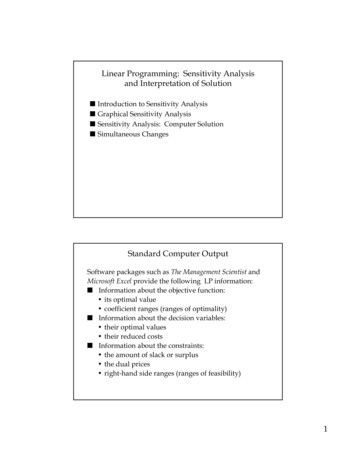
It’s great tohave thewhole ganghelp with alecture.We’re goingto help withtechnicaldetails.This lecture is aboutsensitivity analysis.What happens to theoptimal solutionvalue if one numberin the data ischanged?And we will givesome pointers onhow this can beused in practice.I’m going toask insightfulquestions.I’m goingto becute andsensitive.3

MIT Computer Corporation (mc2)motto: transforming Mass., energizing the worldThe following is a fictional case. It is based onthe DEC case, developed by Rob Freund andBrian Shannahan in 1988.It demonstrates the use of linear programming forplanning the “ramping” of new computerhardware.4

BackgroundMIT Computer Corp (mc2) announced a new family of tabletcomputers and e-readers in the second quarter of 2010.Shipments began in the 3rd quarter of 2010. The tabletcomputers and e-readers had the following code names:– Aardvark. A high-end, general purpose tablet computer, with touchscreen and with large memory disk space.– Bison.A medium-end, general purpose tablet computer with touchscreen– Cougar. A general purpose tablet computer requiring a tablet pen– Deer. A high-end e-reader with many additional functionalities– Emu.An e-reader.The Aardvark required newly developed high speed memory, which was inlimited supply.All of the Bisons, half of the Deers, and 20% of the Aardvarks required anew type of disk drive, which was in limited supply.5

ABCDEAmount(in 1000s)High CapMem. Chips2000040Low CapMem. Chips02221240Avg. # ofnew disk drives.210.5020List Price(in 1000s)1.2.8.6.6.3ItemADemand(in 1000s)18C3Tablets38e-readers326

A Number of Aardvarks manufactured (in 1000s)B Number of Bisons manufactured (in 1000s)C, D, E Maxs.t1.2 A .8 B .6 C .6 D .3 E2A 2B 2C 2D .2 A B .5 DAA B 40E 2402018C 3C 38 32D EA, B, C, D, E 07

Original Spreadsheet: the solutionDecision VariablesProfitConstraintsHigh Cap MemoryLow Cap MemoryNew DrivesMax for AMax for CMax for tabletsMax for indingE32 46.12 in millions3670.82018337.432 binding8

General rule: if there are small changes in the data,the optimal set of basic variables does not 21816.43324169.20.6111111First .8-0.600100-2-1Optimal and final tableau9

The structure of the solution stays thesame with small changes of dataThe basic feasible solution is obtained bysolving linear systems of equations.With small changes in data, we solvealmost the same system. If the RHS changes, the solution andthe optimal objective change linearly. If the cost coefficients change, theoptimal solution stays the same. The sensitivity report puts lots of thisinformation in a useful format.10

Sensitivity Report (SR) Part creaseAllowableDecreaseA1801.21.00E 301.04B16.400.85.20.2C300.61.00E 300.6D0-0.10.60.11.00E 30E3200.31.00E 300.111

Sensitivity Report (SR) Part 2NameHigh CapMemoryLow CapMemoryFinalValueShadow ConstraintPriceR.H. SideAllowableIncreaseAllowableDecrease360401.00E 30470.802401.00E 30169.2New Drives200.8200.616.4Max for A181.04180.7518Max for CMax fortabletsMax fore-readers30.630.6337.40381.00E 300.6320.332169.23212

What is the optimal solution?The optimal solution is in the originalspreadsheet.Decision VariablesProfitA18B16.4C3D0E32 46.12 in millionsIt is also in SR part 1, in the column labeled“final value.”Note: the SR report does not have the profit.13

Troubleshooting tip #1If you see “Lagrange multiplier”instead of “shadow price” in theSR, it is because you forgot toclick on “simplex” as the solver,or you forgot to click on “assumelinear mode” in the former versionof .040.60.6000.30.314

Changes that we will consider1.Change the cost coefficient of a variable2.Change the RHS of a constraint3.–Changing the initial conditions–Purchasing resources at a costIntroducing a new product–Reduced costs15

Why do weneed to use areport? Can’twe just solvethe problemmany timesusing Solver?Solving theproblemmultiple timesis OK for smallspreadsheets,but there areadvantages ofunderstandingthe SR.The SR is a compactway of storinginformation.LP Solvers generatelots of usefulinformation with asingle report.Solving multiple timesis not practical if thereare 1000s ofconstraints.In addition, it isneeded to understandLP theory.TomCathyFinally, it will be onthe first midterm.16

And why aren’t weconsidering changesin the rest of thedata, such as thecoefficients thatmake up the LHS ofconstraints?TomThe SR reports can beused to investigatechanges in thesecoefficients for nonbasicvariables, but not forbasic variables. I’ll tryto explain this once weknow about reducedcosts.Cathy17

Changing the cost coefficient of abasic variablemc2 is uncertain as to whether the Aardvark ispriced to high. They are considering lowering theprice from 1200 to 1000. What will be theimpact on the total revenue?In practice, lowering the priceshould result in an increase indemand. But here we assumedemand is unchanged. In thissensitivity analysis, we changeonly one number in the data at atime, and assume all other data isunchanged.18

The analysis For very small changes in the cost coefficients,the optimal solution is unchanged. Check the allowable increase and decrease of thecost coefficient to see if the solution changes. If the optimal solution is unchanged, then youcan compute the new objective bleIncreaseAllowableDecreaseA1801.21.00E 301.0419

QUESTION FOR STUDENTSSuppose that the list price of the Aardvark ischanged from 1,200 to 11,200. What is the bestanswer below?The sensitivity report says that the optimalsolution will not change.2. The objective value will increase by 180 million.3. The model becomes very inaccurate since itassumes that demand for Aardvarks does notchange.4. All of the above.1.20

Currently, there are no Deer beingproduced. What would be the list priceat which deer would be owableIncreaseAllowableDecreaseD0-0.10.60.11.00E 30 1002. 5003. 700 4. Deer would never be produced1.21

I noticed that the“reduced cost” is thenegative of allowableincrease for D. Is that acoincidence?TomTom, that is not acoincidence. We’llreturn to that later whenwe discuss reducedcosts.Cathy22

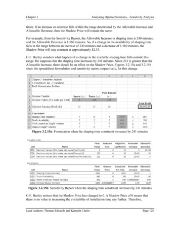
Changing the RHS of a constraint mc2 expects to receive 20,000 new drives.However, the drives are manufactured in acountry experiencing labor strikes. What wouldbe the impact on the optimal solution value if only15,000 new drives were available?We want to find out how the optimalplan would change if the number ofdrives were 15,000.If we learned about labor strikes afterstarting to implement a plan, thingswould be far worse since it is costly tochange a plan after it is implemented.23

Shadow Prices Definition:– The shadow price of a constraint of a linear program isthe increase in the optimal objective value per unitincrease in the RHS of the constraint. VERY IMPORTANT:– The Shadow Price of the i-th constraint is ONLY validwithin the RHS range of thei-th constraint.NameNew DrivesFinalValue20Shadow Constraint AllowablePriceR.H. SideIncrease0.8200.6AllowableDecrease16.424

On the shadow price for new drivesNameNew DrivesFinalValue20Shadow Price .8Shadow Constraint AllowablePriceR.H. SideIncrease0.820AllowableDecrease0.616.4Shadow Price is valid if the RHSnumber ND of new drives satisfies:3.6 ND 20.6The SR report tells how the objective valuechanges, but does not say what the newsolution is.It also doesn’t tell you what happens if theRHS change is not in the allowable range.Nooz25

Question. What is the “increase” in theoptimal objective value if the number ofdisk drives is reduced to 15,000?1.It cannot be determined from the data2. 4,0003.- 4,0004. 4,000,0005.- 4,000,000 6. 12,000,00026

On the demand for tablet computers The total demand for tablets (A, B, C) is currently38,000. What would be the value of increasingthe demand to 40,000, possibly via a marketingcampaign?NameMax fortabletsFinalValue37.4Shadow ConstraintPriceR.H. Side038AllowableIncreaseAllowableDecrease1.00E 300.6If an inequality constraint does not holdwith equality in the optimum solution, theconstraint is non-binding. The shadowprice of each non-binding constraint is 0.27

Question: mc2 is considering an advertizing campaign thatwill increase the demand of Aardvarks to 18,500. The costof the campaign is 400,000. Is it worthwhile?NameFinalValueMax for A18Shadow ConstraintPriceR.H. Yes 2. No3. Cannot be determined from the available data.1.28

Question: mc2 is considering an advertizing campaign thatwill increase the demand of Aardvarks to 20,000. The costof the campaign is 1,000,000. Is it worthwhile?NameFinalValueMax for A18Shadow ConstraintPriceR.H. Yes2. No3. Cannot be determined from the available data.1.29

The real change in Z as the boundon A increases48.548Slope is 047.54746.546181920212230

Midclass Break31

Simultaneous Changes in the RHS One of the forecasters at mc2 is pessimistic aboutthe demand forecasts. One can’t rely on thedemand for A and C to be as high as predicted. Itis much safer to use estimates of 15 and 2. What will be the impact on the optimum objectivevalue if the maximum value of A is reduced to 15and the maximum value of C is reduced to 2?NameFinalValueShadow Constraint AllowablePriceR.H. SideIncreaseAllowableDecreaseMax for A181.04180.7518Max for C30.630.6332

I know this one.There is not enoughinformation to know.TomTom, it turns out that thereis a rule that I haven’tmentioned yet. It’s calledthe 100% rule. And it willhelp answer the questionabout changes of demand.Ella33

A rule for two changes in RHSNameShadowAllowable AllowablePrice R.H.S Increase DecreaseMax for A1.04180.7518Max for C0.630.63CA(-18,0)The red dots arepermissiblechanges.(0,.6)So is the region inyellow.(0,-3)

The 100% for two changes in RHSNameShadowAllowable AllowablePrice R.H.S Increase DecreaseMax for A1.04180.7518Max for C0.630.63100% allowableincrease of C100% allowabledecrease of AThe red dots arepermissiblechanges.100% allowableincrease of A100% allowabledecrease of C35

The 100% rule illustratedC increase.6-18AdecreasePoints satisfyingthe 100% ruleThe red dots arepermissible changes.75Aincrease-3C decrease36

The actual increases in A and C so thatthe basis does not change.C increase.6-18AdecreasePoints satisfyingPointstheat whichthe100% ruleshadow pricesremain validThe red dots arepermissible changes.75Aincrease-3C decrease37

The 100% ruleFor each RHS that changes, compute the amountof change divided by the total allowable change.Add up these fractions. If the total value is lessthan 1, then the shadow prices are valid.NameShadowAllowable AllowablePrice R.H.S Increase DecreaseProposed proposedDecrease /allowableMax for A1.04180.751831/6Max for C0.630.6311/3Total 1/2You can learnmore about the100% rule inSection 3.7 ofAMP.Objective “increases” by-3 1.04 -1 .6 -3.72Revenue decreases by 3.72 million38

Question. Suppose that the Maximum for ADecreased by 1000 (to 17,000), and the Maximumfor C increased by 500 (to 3500). What would bethe increase in the optimum revenue?NameShadowAllowable AllowablePrice R.H.S Increase DecreaseMax for A1.04180.7518Max for C0.630.63It cannot be determined from the data2. - .74 million3. 1.34 million4. - 1.34 million1.39

reaseAllowableDecreaseD0-0.10.60.11.00E 30E3200.31.00E 300.1I’m ready to hearabout reducedcosts. What arethey?There are severalequivalentdefinitions.If you understandreduced costsyou reallyunderstand linearprogramming.40