Transcription
Generation of dense time series synthetic Landsat data through data blendingwith MODIS using a spatial and temporal adaptive reflectance fusion modelThomas Hilker*1, Michael A. Wulder2, Nicholas C. Coops1, Nicole Seitz2, Joanne C.White2, Feng Gao3, Jeffrey G. Masek3, and Gordon Stenhouse41- Department of Forest Resource Management, University of British Columbia, 2424Main Mall, University of British Columbia, Vancouver, British Columbia, V6T 1Z4,Canada2- Canadian Forest Service (Pacific Forestry Centre), Natural Resources Canada,Victoria, British Columbia, V8Z 1M5, Canada3- Biospheric Sciences Branch, NASA Goddard Space Flight Center, Greenbelt MD,20771, USA4- Foothills Research Institute, Hinton, Alberta, T7V 1X6, Canada* corresponding author:Thomas HilkerPhone: 1 (604) 827 4429, Fax : 1 (604) 822 9106, thomas.hilker@ubc.caPre-print of published version.Reference:Hilker, T., Wulder, M.A., Coops, Seitz, N., White, J.C., Gao, F., Masek, J.G.,Stenhouse, G. 2009. Generation of dense time series synthetic Landsat datathrough data blending with MODIS using a spatial and temporal adaptivereflectance fusion model. Remote Sensing of Environment. 113: er:The PDF document is a copy of the final version of this manuscript that wassubsequently accepted by the journal for publication. The paper has beenthrough peer review, but it has not been subject to any additional copy-editingor journal specific formatting (so will look different from the final version ofrecord, which may be accessed following the DOI above depending on youraccess situation).1
AbstractLandsat imagery with a 30 m spatial resolution is well suited for amics. WhileLandsatimages haveadvantageous spatial and spectral characteristics for describing vegetation properties,the Landsat sensor's revisit rate, or the temporal resolution of the data, is 16 days.When considering that cloud cover may impact any given acquisition, this lengthy revisitrate often results in a dearth of imagery for a desired time interval (e.g., month, growingseason, or year) especially for areas at higher latitudes with shorter growing seasons. Incontrast, MODIS (MODerate-resolution Imaging Spectroradiometer) has a hightemporal resolution, covering the Earth up to multiple times per day, and depending onthe spectral characteristics of interest, MODIS data have spatial resolutions of 250 m,500 m, and 1000 m. By combining Landsat and MODIS data, we are able to capitalizeon the spatial detail of Landsat and the temporal regularity of MODIS acquisitions. Inthis research, we apply and demonstrate a data fusion approach (Spatial and TemporalAdaptive Reflectance Fusion Model, STARFM) at a mainly coniferous study area incentral British Columbia, Canada. Reflectance data for selected MODIS channels, all ofwhich were resampled to 500 m, and Landsat (at 30 m) were combined to produce 18synthetic Landsat images encompassing the 2001 growing season (May to October).We compared, on a channel-by-channel basis, the surface reflectance values (stratifiedby broad land cover types) of four real Landsat images with the corresponding closestdate of synthetic Landsat imagery, and found no significant difference between real(observed) and synthetic (predicted) reflectance values (mean difference in reflectance:mixedforestx0.086,0.088 ,broadleafx0.019,0.079 ,coniferous
x0.039,0.093 ). Similarly, a pixel based analysis shows that predicted andobserved reflectance values for the four Landsat dates were closely related (meanr2 0.76 for the NIR band; r2 0.54 for the red band; p 0.01). Investigating the trend inNDVI values in synthetic Landsat values over a growing season revealed thatphenological patterns were well captured; however, when seasonal differences lead to achange in land cover (i.e., disturbance, snow cover), the algorithm used to generate thesynthetic Landsat images was, as expected, less effective at predicting reflectance.Key words: Landsat, MODIS, synthetic imagery, STARFM, data blending, EOSDSubmitted to: Remote Sensing of Environment3
1. IntroductionVegetation canopy biophysical and structural information are required inputs to manylandscape-scale models, including ecosystem process and wildlife habitat models(Peddle et al., 1999; Sellers 1985b; Sellers et al., 1996; Townshend and Justice 1995).Since the launch of the first satellite sensors in the 1970’s, remote sensing has emergedas a key technology for providing modeling inputs in a spatially continuous fashion, withconsiderable progress being made in the determination of biophysical plant propertiesfrom optical sensors (Prince 1991; Prince and Goward 1995; Ecklundh et al., 2001,Patenaude et al. 2005; Masek and Collatz 2006). Key challenges are still imposed bytechnological limitations, requiring trade-offs to be made between the spatial, spectral,and temporal resolutions of an instrument, and often preventing an adequatedescription of ecosystem dynamics and disturbance for modeling purposes. Forinstance, high spatial resolution typically results in a smaller image footprint, or spatialextent, thereby increasing the time it takes a satellite to revisit the same location onEarth (Coops et al. 2006). Conversely, high temporal resolution sensors have a morefrequent revisit rate and produce wide-area coverage with a lower spatial resolution(Holben 1986; Justice et al. 1985).Arguably, the most commonly used satellite sensor for mapping biophysicalvegetation parameters and land cover type is Landsat (Cohen and Goward, 2004). TheLandsat TM and ETM sensors on board the Landsat 5 and 7 platform have a spatialresolution of 30 m, a spatial extent of 185 x 185 km per scene, and proven utility formonitoring land cover and land cover changes (Wulder et al., 2008). Its 16-day revisitcycle, however, which can be significantly lengthened due to cloud contamination (Ju4
and Roy, 2007), can limit Landsat’s use for monitoring biodynamics (Ranson et al.2003; Roy et al. 2008) and may create difficulties in mapping vegetation conditions in atimely manner (Gao et al. 2006; Leckie 1990; Pape and Franklin 2008). The impact ofclouds on satellite imagery can be of major concern (Ju and Roy, 2007), especiallynotably in tropical locations and regions with variable topography. For instance, Leckie(1990) found that the probability of acquiring a cloud-free Landsat scene (cloudcover 10%) can be as low as 10% for some regions in Canada (observed during Julyand August); plus, technical difficulties, such as the scan line corrector failure of theLandsat ETM sensor in 2003 (Maxwell et al., 2007), can further reduce the availabilityof images suitable for analysis.Changes in land cover and ecosystem disturbance are important drivers ofhabitat distribution and species abundance (Pape and Franklin 2008) and as a result, agoal for terrestrial monitoring, especially habitat mapping, is to have both high spatialand temporal resolutions. One possible way to meet this goal is through fusing datafrom sensors with differing spatial and temporal characteristics. In general, data fusionor data blending combines multi-source satellite data to generate information with highspatial and temporal resolution. Several approaches describing existing fusiontechniques are summarized in Table 1. An early example of a fusion model wasillustrated by Carper et al., (1990) who combined 10 m spatial resolution SPOTpanchromatic imagery with 20 m spatial resolution multispectral imagery by using anintensity-hue-saturation (IHS) transformation. The generated composite images havethe spatial resolution of the panchromatic data and the spectral resolution of the originalmultispectral data. Other techniques to enhance the spatial resolution of multispectral5
bands include component substitution (Shettigara, 1992), and wavelet decomposition(Yocky, 1996). One of the first studies designed to increase the spatial resolution ofMODIS using Landsat was introduced by Acerbi-Junior et al. (2006) using wavelettransformations. The algorithm yields classified land cover types and was used formapping the Brazilian Savanna (Acerbi-Junior et al. 2006). Recently, (Hansen et al.2008) used regression trees to fuse Landsat and MODIS data based on the 500m 16day MODIS BRDF/Albedo land surface characterization product (Roy et al., 2008,Hansen et al., 2008) to monitor forest cover in the Congo Basin on a 16 day basis.Table 1: Summary of data blending techniques found in the literature.TechniqueSensor 1IHSTransformsComponentSubstitutionSPOT formsDownscalingMODISCombiningmedium andcoarseresolutionsatellite dataSemi-physicaldata fusionapproachusing MODISBRDF/AlbedoSTARFMScale 1(m)10Sensor 2Spot XSScale 2(m)202030SPOT PanSPOT Pan1010Carper et al.,1990Shettigara,199228.5-120SPOT Pan10Yocky, 1996MODIS 1,2MODIS 3-7MODIS 1,2250500250LandsatTMMODIS 3-730MODIS250LandsatTM30Acerbi et al.,2006Trishschenkoet al., 2006Busetto etal., 2007MODIS500LandsatTM30Roy et al.,2008,Hansen etal., 2008MODIS500LandsatTM30Gao et al.,2006XS SPOTLandsatTMLandsatTM500Author*Pan Panchromatic, XS Multi-spectral6
While there are numerous examples existing in the current literature that fusedata from multiple sensors, only a few techniques yield calibrated outputs of spectralradiance or reflectance (Gao et al., 2006), a requirement to study vegetation dynamicsor quantitative changes in reflectance over time. The Spatial and Temporal AdaptiveReflectance Fusion Model (STARFM) (Gao et al., 2006) is one such model and wasdesigned to study vegetation dynamics at a 30 m spatial resolution. STARFM predictschanges in reflectance at Landsat’s spatial and spectral resolution using high temporalfrequency observations from MODIS. STARFM predicts reflectance at up to daily timesteps, depending on the availability of MODIS data. MODIS sensors are present on thepolar orbiting Terra and Aqua spacecrafts, launched in 1999 and 2002 respectively, andacquire data in 36 spectral bands, 7 of which are commonly used for terrestrialapplications (Wolfe et al. 2002). Depending on the spectral channel of interest, MODIShas spatial resolutions of 250 m, 500 m, and 1 km at nadir, with near daily globalcoverage.STARFM was initially tested to predict daily Landsat-scale reflectance in the redand NIR region using the 500-m daily surface reflectance product (MOD09GHK) withone or more pairs of Landsat and MODIS images acquired on the same date (T 1) andone or more MODIS observations from the prediction date (T 2) (Gao et al., 2006). Formore humid areas of the Earth, which are frequently cloud contaminated, it can,however, be useful to base the predictions on multi-day composites, such as providedby the 8-day MOD09A1/MYD09A1 product, to minimize cloud contamination in existingMODIS scenes (Vermote, 2008). Spectral information from the Landsat ETM sensor is7
synthesized by matching the locations of Landsat ETM bands 1-5 and 7 to theircorresponding MODIS land bands (Table 2) (Gao et al., 2006).Table 2: Comparison spectral bands Landsat and MODIS.LandsatMODISBandSpectral rangeBand nameBandSpectral range1450-520 nmBlue3459-479nm2520 – 600 nmGreen4545-565nm3630-690 nmRed1620-670nm4760-900 nmNear IR2841-876nm51550-1750 nmMid IR61628-1652nm72080-2350 nmMid IR72105-2155nmIn the study presented herein, we build upon the work of Gao et al. (2006) andinvestigate the suitability of the STARFM algorithm for generating synthetic Landsatimages that may then be used to investigate vegetation dynamics in different land covertypes. We assess the quality of the synthetic (predicted) Landsat reflectance values fora number of broad vegetation classes (mainly coniferous forest), by comparing thesepredictions with reflectance values from real (observed) Landsat images acquiredthroughout one growing season. The objective of this study is to investigate thepotential of STARFM for assessing seasonal changes (i.e. changes due to vegetationgreen up and leaf senescence) in vegetation cover and vegetation status in the borealand sub-boreal forest regions for which the potential of acquiring frequent higher spatialresolution data (and therefore the potential for mapping of vegetation dynamics) isotherwise low. Algorithms like the one used in this study are important components of8
current research efforts seeking to map high spatial resolution changes in vegetationcover and status with high temporal density, over larger areas. Data blendingapproaches, such as STARFM can help minimizing the technical limitations and tradeoffs associated with information needs that require data with both high spatial and hightemporal resolutions. Applications such as monitoring seasonal changes in vegetationbiophysical and structural attributes over large areas can benefit from the synergies ofmultiple data sources such as MODIS and Landsat. Advances in data blending can alsoinfluence the design of new sensors, where the advantages of different spatial andtemporal resolutions may be fully realized in the creation of different sensors ondifferent platforms, with the complementary nature of these systems in a data blendingapproach, considered from the outset of the design process.2. Methods2.1 Study area and image dataCriteria for site selection included the availability of four or more consecutive Landsatimages in the growing season of a given year with less than 10% cloud cover. Our studyarea is the Landsat WRS-2 Path 47 / Row 24, centered at approximately 51o 41’ 00” Nlatitude and 121o 37’ 00” W longitude, located in central British Columbia, Canada(Figure 1). The 185 x 185 km study area intersects with the 100 Mile House and CentralCariboo Forest Districts of the Southern Interior Forest Region. The vegetation in thisarea is dominated by coniferous tree species, including Douglas-fir (Pseudotsugamenziesii, Mirbel), lodgepole pine (Pinus contorta var. latifolia, Douglas ex Loudon) andwhite spruce (Picea glauca, (Moench) Voss). The climate in this area is extreme, with9
characteristically hot, moist summers and cold winters, which often have large amountsof snow accumulation (Meidinger and Pojar, 1991).10
2Figure 1: Map of the study area. The study site encompasses a Landsat scene (185 x 185 km near WilliamsLake BC, Canada11
Five cloud-free Landsat scenes acquired between May and mid October 2001were available for the study site and were acquired through the USGS GLOVIS portal(http://glovis.usgs.gov/). Images were atmospherically corrected using the cosineapproximation model (COST) (Wu et al., 2005) and radiometrically normalized (Hall etal. 1991b) with respect to the 2005 imagery in order to simplify the comparison betweenthe data. The registration accuracies (RMS error) for the five Landsat scenes were 0.47m for the image acquired May 6, 2001 and 0.49 m for the images acquired July 9, Aug10 and Sept 27, 2001.Additionally, 19 eight-day MODIS composites (MOD09A1, using data from theTerra platform) for the same time period and with a spatial resolution of 500 m wereobtained from the EOS data gateway of NASA’s Goddard Space Flight Center(http://redhook.gsfc.nasa.gov). Figure 2 contains an overview of the Landsat andMODIS scenes used in this study. Following STARFM algorithm input requirements, theMODIS data were reprojected to the Universal Transverse Mercator (UTM) projectionusing the MODIS reprojection tool (Kalvelage and Willems 2005), clipped to the extentof the available Landsat imagery, and resampled to a 30 m spatial resolution using anearest neighbour approach.12
Figure 2: Acquisition dates of Landsat and MODIS scenes used for this study. Note that MODIS data wereacquired as 8-day composites, the dates given in the figure are the first day of the 8-day acquisition period,respectively.13
2.2 Land cover classificationA Landsat derived land cover classification product developed by the Earth Observationfor Sustainable Development of Forests (EOSD) initiative, a joint collaborative betweenthe Canadian Forest Service and the Canadian Space Agency, provided information onland cover types in the study area (Wulder et al., 2003). The EOSD product is basedupon the unsupervised classification, hyperclustering, and manual labelling of Landsatdata, facilitating the classification of land cover types over larger areas (Franklin andWulder, 2002; Slaymaker et al., 1996; Wulder et al., 2003). The EOSD productrepresents 23 unique land cover classes mapped at a spatial resolution of 0.0625 ha(equivalent to a 25 m by 25 m pixel) thereby representing circa year 2000 conditions(Wulder et al., 2008). The accuracy of the EOSD product was found to be 77%,achieving a target accuracy of 80%, with a 90% confidence interval of 74 – 80% (formore detailed information see Wulder et al., 2007).EOSD land cover data for the study area were downloaded from the EOSD dataportal (http://www4.saforah.org/eosdlcp/nts prov.html) and resampled to a 30mresolution using a nearest neighbour approach. The dominant land cover type in thestudy area is coniferous forest (comprised of Douglas-fir, lodgepole pine, and whitespruce) with subsidiary herbal and shrub vegetation and patches of water and rocks.Land cover patches are generally large, the landscape can, however, be quiteheterogeneous within some areas due to harvesting activities and related cut-blocksand access road networks. About 1.8% of the study area has not been classified due to14
cloud contamination during acquisition of the Landsat scene used for EOSDclassification.This area has been excluded from data analysis. The classificationaccuracy for coniferous and deciduous forests and their associated density classes is 92%, the mixed forest class is classified with 88% accuracy (Wulder et al., 2003).2.3 Data processing using STARFMSTARFM predicts pixel values based upon a spatially weighted difference computedbetween the Landsat and the MODIS scenes acquired at T 1, and the Landsat T1-sceneand one or more MODIS scenes of prediction day (T2), respectively (Gao et al., 2006). Amoving window technique is used to minimize the effect of pixel outliers therebypredicting changes of the center pixel using the spatially and spectrally weighted meandifference of pixels within the window area (Gao et al., 2006). The prediction algorithmin STARFM is given by (Gao et al., 2006),wwL xw / 2 , yw / 2 , T2Wij M x i , y jT2L x i , y jT1M x i , y jT1(1)i 1 j 1where L xw / 2 , y w / 2 , T2 is a Landsat pixel value predicted for the time T2, w is the size ofthe moving window and xw/2, yw/2 is the central pixel within this moving window. Thespatial weighting function Wij determines how much each neighbouring pixel (xi,yj) in wcontributes to the estimated reflectance of the central pixel. M x i , y jT2 is the MODISreflectance at the window location ( xi , y j ) observed at T2, while L xi , y jT1andM xi , y jT1 are the corresponding Landsat and MODIS reflectance values observed atthe base date T1, respectively (Gao et al., 2006). The weighting function implemented inSTARFM (when based on a single Landsat and MODIS image as T 1 input) is calculated15
from the product ( Cij ) of the spectral (Si,j) and spatial distance (Di,j) between the centralpredicted pixel and the surrounding candidate pixel. Wij is calculated as the normalizedreverse function of this product (Gao et al., 2006).wWi , jw1 / Cij /1 / Cij(2)i 1 j 1An area of 1500 m x 1500 m was selected as the moving window size forSTARFM predictions (Gao et al., 2006). The uncertainties of Landsat and MODISsurface reflectance were set to 0.002 and 0.005 for the visible and the NIR bands,respectively (Gao et al., 2006). Synthetic Landsat images were predicted using theLandsat scene acquired at 2001/08/10 in conjunction with the MODIS scene acquired at2001/08/13 as T1 data. T2 was defined as the dates for which the remaining 18 MODIS8-day composites were available. The August MODIS and Landsat image pair wasselected as T1 input because it had the least amount of cloud cover (close to 0%), andbecause the temporal difference between the MODIS and the corresponding Landsatscene was minimal (reducing the likelihood for changes in land cover resulting fromharvesting or phenological changes).Clouds in Landsat data were flagged by means of a cloud mask algorithm (Irish2000; Irish et al., 2006), which uses subsequent filtering techniques to identify cloudcontamination in Landsat data based on pixel brightness, surface temperature andseveral band ratios to eliminate highly reflective vegetation, senescing vegetation, andhighly reflective rocks and sands (Irish 2000; Irish et al., 2006). Clouds in the MODISimagery were identified using the MODIS quality flags. Low quality pixels (such as snow16
or cloud contaminated) in either Landsat or MODIS data were predicted in STARFM butexcluded from the statistical analysis.2.4 Assessment of STARFM synthetic Landsat imageryThe four remaining Landsat scenes were used for validation (cross-comparison) toallow assessment of the quality of the STARFM predictions (real to synthetic Landsatimages) made throughout the 2001 growing season. The prediction accuracy wasassessed on a per pixel basis by comparing the reflectances of observed and predictedLandsat images for a subset of the study area (random sample of 10% of the vegetatedland surface area). The prediction quality of STARFM was assessed from the differencebetween observed and predicted scenes by comparing the 4 image pairs on a pixel bypixel basis and per land cover type defined from the EOSD land cover product. A twosided t-test of the difference images was used to determine whether there is astatistically significant difference between observed and predicted reflectance values(i.e., whether the mean difference between observed and predicted data variedsignificantly from zero).Changes in vegetation green-up and leaf-down were described using the normalizeddifference vegetation index (NDVI) (Tucker 1979), as one of the most commonly usedmeasures of vegetation cover and leaf area (Asrar et al., 1984; Daughtry et al., 1983;Myneni and Williams 1994; Sellers 1985a). NDVI was calculated per land cover class17
for all 18 prediction dates and then compared to the Landsat observed NDVI values atthe 4 validation dates throughout the 2001 growing season.3. ResultsTable 3 shows the percent coverage of the different land cover types found withinthe study area. The majority of land is covered by open and sparse coniferous forest,while mixed and broadleaf forest types only cover about 4% of the study area. TheSTARFM algorithm yielded 18 high spatial resolution, synthetic Landsat images for the2001 growing season (May through October) using a Landsat and a MODIS sceneacquired in August 2001 as the T1 images, and 18 eight-day MODIS compositesbetween May and October 2001 as the T2 images for prediction. Figure 3 shows the fiveobserved Landsat scenes (4A, 4D, 4G, 4J, 4M), the corresponding MODIS compositesused for STARFM predictions (4B, 4E, 4H, 4K, 4N), and the predicted synthetic Landsatimages in the right column (4C, 4F, 4L, 4O). No image was synthesized for August 13,as the August imagery was used as T1 input. Larger, visible differences in Figure 3 weredue to cloud contamination in the Landsat and MODIS scenes and, in the case of theMay image, snow cover. The quality of the synthetic Landsat images was affected bycloud contamination in the T2 MODIS composites, resulting in a few streaking effects inthe synthesized images, particularly in the shorter wavebands (Figure 3C and O, upperportion of the image). Figure 4 shows an example of a 10 x 10 km subset of the Landsatscene obtained in July (Figure 4A) and the corresponding STARFM synthetic image(Figure 4B). STARFM maintained a high level of spatial detail in the predicted scenes,including areas with more heterogeneous and complex land cover types. The spatial18
patterns related to differing land cover types were well maintained in the syntheticimages (Figure 4). Figure 5A-L shows a per-pixel comparison between observed andpredicted Landsat reflectance for the focus area shown in Figure 4. The rows representthe reflectance values for the NIR, red and green TM band, respectively, the columnsrepresent the four validation dates (May 9, July 12, September 30 and October 08).Highest correlations between observed and predicted pixel values were found for theNIR band (0.73 r2 0.82; p 0.01) (Figure 5A-D), while the shorter wavebands in thevisible part of the spectrum yielded weaker relationships. The coefficients ofdetermination ranged between 0.27 r2 0.67 for the red and between 0.44 r2 0.62 forthe green band. Prediction accuracy was highest for the scenes predicted for July 12and September 30 (Figure 5B-C, F-G and J-K), while the precision was lower especiallyfor the visible bands at the beginning of the vegetation period (Figure 5 E,I). Therelationship between observed and predicted pixel values closely followed the 1-to-1line (Figure 5 A-L) thereby showing that Landsat reflectance was accurately predictedby STARFM. Some deviations from this 1-to-1 line, however, were found for the redband towards the end of the vegetation period (Figure 5H). Table 4 shows a pixel basedcomparison between observed and predicted Landsat images for TM bands 2-5 andNDVI summarized for the most important land cover categories, 1) shrub and herb, 2)forested vegetation and 3) all landcover types combined. The first column in each subtable is showing the coefficient of determination for the pixel based regression betweenthe observed Landsat scenes (May 06, July 09, Sept 27 and Oct 05) and the STARFMpredicted images that whose prediction date was closest to the observed scenes (May09, July 12, Sept 30 and Oct 08, respectively). The relationship between observed and19
predicted was highest for the longer wavebands (Red, NIR and SWIR, NDVI), and forthe more heterogeneous land cover types, showing a larger range of pixel values. Thesecond column is showing the intercept of the relationship, data were normalized to themaximum observed reflectance of each band in order to facilitate a comparisonbetween different wavelengths. STARFM consistently overestimated the intercept bybetween 0 and 19% of the observed reflectance, best results were found for the longerwavelengths. The slope between observed and predicted pixel values followed the 1:1line relatively close but the predicted values slightly underestimated the observedreflectance in all cases. Best results were found for NDVI band, likely due to thenormalization of the indexed values.2Table 3: EOSD-Landcover types and percent coverage found within the study area (185 x 185 km ).Land cover typeShadowWaterSnow/IceRock/RubbleExposed LandBryoidsShrub TallShrub LowWetlandHerbConiferousBroadleafMixed forest% 2.251.5820
Table 4: Pixel based regression of the observed Landsat scenes (May 06, July 09, Sept 27 and Oct 05) versusthe STARFM predicted images whose prediction date was closest to the observed scenes (May 09, July 12,Sept 30 and Oct 08). The first column in each sub-table is showing the coefficient of determination, thesecond column is showing the intercept, normalized to percent total reflectance of the observed image (forinstance a value of 0.1 means the predicted image overestimated the reflectance by 10%), the third column isshowing the slope of the relationship between observed and predicted.LandcoverTMbandMay 062r2aJuly 09br2aSept 27br2aOct 05br2abHerb/shrub0.55 0.03 0.93 0.67 0.09 0.82 0.66 0.07 0.84 0.69 0.12 0.78Forest0.42 0.14 0.69 0.57 0.13 0.77 0.59 0.12 0.78 0.64 0.10 0.78Combined0.47 0.09 0.77 0.60 0.11 0.76 0.61 0.10 0.80 0.65 0.12 0.77Landcover3r2abr2abr2abr2abHerb/shrub0.61 0.05 0.90 0.70 0.09 0.83 0.68 0.09 0.84 0.64 0.12 0.78Forest0.53 0.12 0.74 0.63 0.11 0.79 0.69 0.10 0.83 0.73 0.09 0.84Combined0.56 0.09 0.80 0.66 0.10 0.80 0.69 0.08 0.83 0.69 0.09 0.82Landcover4r2abr2abr2abr2abHerb/shrub0.79 0.04 0.90 0.85 0.04 0.92 0.75 0.07 0.87 0.73 0.07 0.85Forest0.47 0.16 0.70 0.59 0.12 0.78 0.51 0.14 0.79 0.51 0.16 0.78Combined0.71 0.07 0.85 0.78 0.06 0.88 0.67 0.08 0.81 0.67 0.10 0.80Landcover5r2abr2abr2abr2abHerb/shrub0.82 0.03 0.90 0.85 0.05 0.92 0.73 0.07 0.86 0.53 0.19 0.73Forest0.76 0.07 0.86 0.80 0.05 0.89 0.70 0.08 0.82 0.62 0.13 0.75Combined0.81 0.05 0.90 0.83 0.05 0.90 0.70 0.07 0.84 0.61 0.14 0.71LandcoverNDVIr2abr2abr2abr2abHerb/shrub0.84 0.04 0.88 0.93 0.04 0.92 0.91 0.06 0.86 0.85 0.08 0.82Forest0.50 0.08 0.86 0.84 0.14 0.92 0.64 0.13 0.74 0.82 0.15 0.86Combined0.67 0.10 0.80 0.83 0.04 0.91 0.80 0.06 0.87 0.80 0.05 0.9021
Figure 3: Comparison between observed Landsat scene (left column), observed MODIS scene (centralcolumn) and predicted Landsat scene (right column) for the 5 acquisition dates. No synthetic data has beenpredicted for August 13 as the Landsat input data from August have been used as T 1 image (Bandcombination: NIR, Red, Green).22
Figure 4: Comparison of fine scale structure between observed Landsat scene (acquired July 09 2008) andpredicted Landsat scene (predicted using July 12 as prediction date). STARFM was able to represent theheterogeneity of Landscape well.23
Figure 5: Per-pixel comparison between observed and predicted Landsat reflectance. The rows represent thereflectance values for the NIR, red and green TM band, respectively, the columns represent the fourvalidation dates. Highest correlations between observed and predicted pixel values were found for the NIRband (0.73 r2 0.82; p 0.01) (Figure 5A-D), while the visible reflectances yielded weaker relationships22(0.27 r 0.67 for the red (Figure 5E-H), and 0.44 r 0.62 for the green band (Figure 5I-L)) (p 0.01). Predictionaccuracy was highest for the scenes predicted for July 12 and September 30 (Figure 5B-C, F-G and J-K),while the accuracy was lower especially for t
2008) used regression trees to fuse Landsat and MODIS data based on the 500m 16-day MODIS BRDF/Albedo land surface characterization product (Roy et al., 2008, Hansen et al., 2008) to monitor forest cover in the Congo Basin on a 16 day basis. Table 1: Summary of data blending techniques found in the literature.