WIXLIB

Insurance ProductRecommendationSystemKailan Shang, FSA, CFA, PRM,SCJPRecommending an appropriate insurance productis important for insurers to acquire new businessfrom either a new client or an existing client. Theclient’s demographic and financial information isuseful for predicting the most wanted insuranceproduct type. With the right recommendation, theprobability of completing a sale will be higher andthe length of time to make a sale can be shortened.Traditionally, insurance agents have used householdfinancial planning to help clients choose insuranceproducts. However, it requires significant time, skilland experience on the agent’s part. Other distributionchannels such as telemarketing may not provide theopportunity to conduct such a complicated analysis forcustomers. On the other hand, insurance companieshold relevant information that is very helpful forpredicting the next likely sale to a client.Business CaseA life insurance company wanted to improve theeffectiveness of its selling efforts to reduce cost andincrease sales volume. The company has millionsof existing policyholders, and it had established apartnership with another financial institution thatallows cross-selling. Demographic information,purchase history, financial information and claiminformation on existing customers are available.The company was interested in knowing the mostlikely product that a client would purchase and theprobability that the sale would be completed.DataFive categories of data are used for the project:1.Demographic information including age, gender,address, ZIP code, smoker/nonsmoker, healthstatus, occupation, marital status and informationabout dependents2.3.4.5.Financial information including assets, realestate, income, loans and spendingPurchase history including product type, productname, issue age, face amount, premium rate, faceamount change, partial withdrawal, policy loanand product conversionClaim history including time, amount, payment, etc.Communication history including last contacttime, reason, outcome, complaints, etc.For categorical variables such as address, ZIP code andcommunication reasons, dummy variables are createdto represent them. The data are not complete for allclients. For missing demographic or financial data, thevalue in the most similar record is used. The similarity ismeasured by the Euclidean distance given byn(Yi — Xi )2 i li 1whereX is the data record with missing value for variable l.Y is a complete data record in the data set.n is the number of variables in the data set.ModelsGiven the large amount of explanatory variables and thecomplicated relationships, traditional linear andnonlinear regression models that require exact modelspecification are not suitable. An artificial neural network(ANN) model was chosen to estimate the probability ofnew insurance purchases. ANN models mimic humanneural networks, which are capable of makingcomplicated decisions with layers of neurons. ANNmodels can approximate complicated relationshipswhose model specifications are unknown. A multilayerfree-forward neural network model was used for theestimation. Figure 1 shows the model structure.Notes:1. A sigmoid function is used for specifying therelations between layers,1g(x) 1 e-x .2. Each node in the network is determined by theii–1i–1nodes in the previous layer, aj g ( 0j x a ) , whereaji is node j in layer I, and a i–1 is a column vectorincluding all the nodes in the previous layer, where0j i–1 is a row vector including the weights for all thenodes in layer i 1 for estimating aji .6

Insurance Product Recommendation SystemFigure 1 ANN Model Structurea 00a01a 20a 01a 021121aaa 21a 220a n–2a 31a 320a n–1a 41a 42a 03a 13a 23a n0Input g (1)DataHidden g (3)LayerHidden g (2)LayerOutputThe first layer is the input data. The second and thirdlayers are hidden layers. The fourth layer is the outputlayer, which comprises the probabilities of buying eachof three insurance products. Back-propagation withrandom initialization of model parameters is used totrain the ANN. For some nodes in the second layer, notall the input data (first layer) are used to determinetheir values. As shown in Figure 2, expert opinionsFigure 2 Heuristic Training for theSecond LayerDemographicInfoFinancial InfoPurchaseHistorya 01Affordabilitya 11Risk Appetitea 21Satisfactiona 31New Insurance NeedsClaim HistoryCommunicationHistoryare used to construct part of the second layer. Fournodes are used to represent the affordability, riskappetite, client satisfaction and new insurance needsdetermined by selected subsets of input data. Experts’inputs on the weights ( 0j0 , j 0 to 4) of input data forthe four nodes are used for parameter initialization. Theremaining node a41 in the second layer is assumed tobe affected by all input data to allow model flexibility.Some existing customers had already bought two ormore products. They are used as the positive examplesin the calibration and are the key to predicting thelikelihood of buying a second product and its mostlikely type. The data set was divided randomly intotraining data and validation data. The calibrated modelbased on the training data was validated using severalpractical approaches. For example, the ANN outputs fora customer who has bought a universal life (UL) productare that the customer has a probability of 80%, 30%and 50% to buy a new term life (TL), new UL andlong-term care (LTC) product, respectively. Therefore,the recommended product is TL. The 10 most similarcustomers with two or more products including at leastone UL product are sought. If no fewer than 50% (80%/[80% 30% 50%]) of the 10 customers have bought a TLproduct, the ANN model is considered reasonable. Thesimilarity is measured using Euclidean distance. Becauseof the large number of input variables, the impact ofimportant variables could be diminished by unimportantvariables if equal weights are applied. The four nodes inthe second layer (affordability, risk appetite, satisfactionand new insurance needs) are used instead to determinethe similarity of customers. Using the validation data,the model has a reasonable rate of 69%.The model was also validated using a pilot salesproject by contacting around 2,000 existing customerswith only one insurance purchase in the past. Thesecustomers are those with a high chance of purchasinga second product as predicted by the ANN model.The success rate of selling a second product is 4.5%compared to a past average level of 1.3% when theselection of contacted customers was based onqualitative analysis targeting high-net-worth clients.The 4.5% success rate is lower than expected based onthe model prediction, with possible reasons includingchanges in family and financial conditions and havingmade purchases with other insurers.7

Insurance Product Recommendation SystemResultsThe ANN model was used to estimate the most likelyproduct to be bought and the probability of completingthe new sale for each existing customer. The customerswere then ordered by the probability. Table 1 shows thepercentage of customers who will buy a product witha probability higher than a certain value based on themodel result. For example, 3% of the existing customerswill buy an LTC product with a probability of 50%.Using these results, existing customers can be contactedwith relevant product information. The cost can also bemanaged by limiting the selling efforts only to customerswith a high probability of completing the sale. The modelcan be further enhanced by estimating the cost and faceamount of a product that a customer is likely to accept.Table 1 ANN Result Summary for aSample Data C2%3%6%Kailan Shang, FSA, CFA, PRM, SCJP, is co-founder ofSwin Solutions Inc. He can be reached at kailan.shang@swinsolutions.com.8

Machine Reserving:Integrating MachineLearning Into YourReserve EstimatesDale Cap, ASA, MAAAgathering data and engineering features from the data,and building and evaluating the models. As in theactuarial control cycle, it is important to continuallymonitor results.Through our research, we have found significantimprovements in the prediction of reserves by employingthis ML process. Overall we have found a reduction inthe standard and worst case errors by 10%. To assistactuaries in testing the value of ML for themselves, thispaper will provide an outline of the ML process.Define the ProblemTwo hundred years ago a captain may have had only asounding line and his experience to navigate throughuncharted waters. Today a captain has access to manyother data sources and tools to aid in his navigation,including paper charts, online charts, engineeringsurveys, a depth sounder, radar and GPS. These newtools don’t make the old tools obsolete, but anymariner would be safer and more accurate in theirpiloting by employing all the tools at their disposal.In the same vein, actuaries who solely use traditionalreserving techniques, such as triangle-based methods,aren’t capitalizing on new technologies. Actuaries shouldstart adopting other techniques such as machine learning(ML). ML is a field of predictive analytics that focuses onways to automatically learn from the data and improvewith experience. It does so by uncovering insights in thedata without being told exactly where to look.ML is the GPS for actuaries. As GPS improvednavigation, ML has the potential to greatly enhanceour reserves. It is important to note though that ML isnot just about running algorithms; it is a process. At ahigh level this process includes defining the problem,Similar to the Actuarial Control Cycle, the first step is todefine the problem. In our context, we are interestedin efficiently calculating the unpaid claims liability(UCL). We want to calculate this quantity in an accuratemanner that minimizes the potential variance in theerror of our estimate.Actuaries often use various triangle-based methods suchas the Development and the Paid Per Member Per Month(Pd PMPM) to set reserves. These methods in principleattempt to perform pattern recognition on limitedinformation contained within the triangles. Although thesemethods continue to serve actuaries well, informationis being left out that could enhance the overall reserveestimate. To make up for the lack of information used toestimate the reserves, an actuary relies heavily on his orher judgment. Although judgment is invaluable, biasesand other elements can come into play, leading to largevariances and the need for higher reserve margins.As described in our prior article1, the range of reserveestimate error present in company statements pulledfrom the Washington State Office of the InsuranceCommissioner website was 10% to 40%. ThisFigure 1 Machine Learning ProcessDefine theProblemData & FeatureEngineeringModeling &EvaluatingResults1 Cap, Coulter, & McCoy, 20159

Machine Reservingrepresents a wide range of error and has significantimplications, including an impact to the insurer’srating status, future pricing and forecasting decisions,calculation of premium deficiency reserves, or evenunnecessary payout of performance bonuses.Data and Feature EngineeringGathering data is something that actuaries are alreadygood at. Leveraging off their expertise along with othersubject matter experts will be helpful in identifying allavailable sources for use. There is often a saying withML that more data often beat a sophisticated algorithm.Once the data have been gathered, the actuary willneed to engineer the data to improve the model’spredictive power. This is referred to as featureengineering and can include the transformation,creation, conversion or other edits/additions to thedata that will benefit the process. As an example,suppose we were estimating the cost of a housewith only two fields: the length and the width of thehouse. We could help improve the model by featureengineering a new feature called square footage, wherewe would multiply the length and width.The gathering and engineering of the data can be a difficultstage to get through, and without the right people on theteam, it could lead to a wasted effort. Having domainknowledge on the team enables a more thoughtfulconsideration of what sources and features are important.In our research we have found many features that havepredictive power for reserve setting. The following is asample list of features that could provide value: SeasonalityNumber of workdaysCheck runs in a monthLarge claimsInventoryInpatient admits/daysMembership mix by productChange in durationCost-sharing componentsDemographicsPlace of serviceModeling and EvaluatingOnce the data have been prepared, the user will applyvarious ML models to the data set. In general, there aretwo types of data: the training set and the testing set.Figure 2 Supervised Machine LearningIncurredMonthLagArea MonthWorkdaysCheckRunsIncurred Age/Inventory & PaidGenderOtherActualFeatures IncurredJan -10xxxxxxxx250.00Jan -10xxxxxxxx240.00Jan -10xxxxxxxx265.00Jan -10xxxxxxxx280.00Jan �——Dec -11xxxxxxxx335.00Dec -11xxxxxxxx305.00WorkdaysCheckRunsxxIncmoDec -12LagArea MonthxxMLModelIncurred Demo- OtherExpectedInventory & Paidgraphic Features Incurredxxxx250.0010

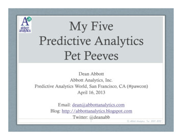
Machine ReservingThe training set is the data used to train and crossvalidate the model and comprises historical data (inthe case of reserving, historical completed data). Thetesting data on the other hand include only the datafrom which you wish to derive predictions (for example,the current month’s reserve data).These results were then compared against typicaltriangle-based methods, where we tested the percentagerange of UCL error over 24 different reserving months.Overall we found that ML added significant value inreserve setting, and we highly encourage reservingteams to explore this process for themselves.To evaluate the model, a portion of the training set iswithheld in order to cross-validate the results. The modelsthat are identified to perform well on the withhold set arethen applied to the testing data to create the predictions.ConclusionPredictive analytics are not new to actuaries. Methodslike these are fairly common on the casualty side andhave recently become more popular within health carefor predicting fraud, readmission and other aspects.However, those within health care are often being ledby data science teams, who continue to fill a largeranalytics role within the health space. It is only a matterof time before these techniques become standard toreserving. The question is: Who will fill this role? Willactuaries stay at the helm, or will we transfer some ofour functions to data science teams?There are many different machine learning models, eachof which has its own strengths and weaknesses. Thusthere is no one model that works best on all problems.ResultsFor our research we used supervised learning techniquesclassified as regression. We ran various ML models anddetermined which ones were the most appropriate forthe problem based on cross-validation techniques. Wethen used an ensemble method to blend the variousmodel outputs for an overall prediction. An example ofthis type of technique can be found in our prior article2.We hope that the process outlined above will providesome guidance and at least prepare actuaries for theirfirst steps in this space.Figure80% 3 UCL Prediction Error Range (Box and Whisker Plot)60%Prediction Error Range40%20%0%xxxxxxModel 1Model 2xxModel 5Linear Stacking–20%–40%Paid PMPMDevelopmentModel 3Model 4–60%Triangle BasedMachine Learning ModelsEnsemble2 Cap, Coulter, & McCoy, 201511

Machine ReservingAppendixTriangle BasedStatisticsMean ErrorStandard ErrorKurtosisSkewCumulative ErrorWorst ErrorPaidPMPMMachine Learning ModelsDevelopment Model 1Model 2EnsembleModel 3Model 4Model 7.6%49.1%57.7%29.0%41.1%28.5%31.4%27.0%25.3%Dale Cap, ASA, MAAA, is an actuary with a passion foranalytics. He can be reached at dale j cap@outlook.com.12

Variable SelectionUsing ParallelRandom Forestfor MortalityPrediction in HighlyImbalanced DataMahmoud Shehadeh,Rebecca Kokes, FSA, MAAA andGuizhou Hu, M.D., Ph.D.In the last few years, the industry has startedmoving away from traditional actuarial methodstoward more statistically sound methodologiesincluding parametric and nonparametric approachessuch as generalized linear models and machinelearning algorithms to better assess risks. Usingsuch techniques and utilizing the full potential ofunderwriting data can improve mortality predictiongreatly. In the life insurance industry, actuaries andunderwriters need to process a substantial amount ofdata in order to assess the mortality of applicants asquickly and accurately as possible. Examples of suchdata include, but are not limited to, demographic,paramedic and medical history. The data can benumerical (age, face amount), categorical (gender,smoking status) and even free text. However, usingsuch data is not always straightforward.In this article we present a practical example of theintersection of life insurance, machine learning and bigdata technology. The aim is to use a random forest (RF)algorithm to identify the most important predictors(from a set of hundreds of variables) that can be usedin mortality prediction, that is, to reduce number ofvariables from hundreds to dozens while retainingthe predictive power. In addition, the use of parallelcomputing to speed the process and stratified samplingto deal with highly imbalanced data is discussed.1The medical history of applicants includes hundreds,if not thousands, of unique keywords that have thepotential to increase the accuracy of risk assessment.Typically, one can include this information as predictorsin regression analysis following two approaches: first,by manually selecting the most important terms

predictive analytics to provide solutions in their work. Let us know your thoughts and share other examples of predictive analytics in action at the SOA Engage Research Community, our new online forum for discussing ideas. R. Dale Hall, FSA, CERA, CFA, MAAA Managing Director of Research Society of Actuaries 3 Comparing Policyholder Efficiency