Transcription
Mixed-effects Regression Modelsfor Longitudinal Dichotomous DataChapter 91
Logistic Regression - model that relates explanatory variables(i.e., covariates) to a dichotomous dependent variableMixed-effects Logistic Regression - model that relates covariatesto a dichotomous dependent variable, where observations arenested Longitudinal: repeated observations within subjects Clustered: subjects within clustersmodels can also be recast as probit regression models2
Logistic Regression Model with dichotomous xgroupxcontrol0treatment 1 Y response0160303060prob1/32/3odds1/22logit-.693.693 P r(Yi 1) βlog 0 β1xi1 P r(Yi 1) exp β0 odds of response for x 0 (30/60 1/2)β̂0 log(1/2) .693exp(β0 β1) odds of response for x 1 (60/30 2)β̂0 β̂1 log(2) .693β̂1 .693 .693 1.3863
odds ratio ratio of odds per unit change in xexp(β̂0 β̂1) exp(β̂0) exp(β̂1) exp(1.386) 44
Model is not linear in terms of the probabilitiesexp(β0 β1xi)1 P r(Yi 1) 1 exp[ (β0 β1xi)]1 exp(β0 β1xi)5
Model is linear in terms of the logits P r(Yi 1) βlog 0 β1xi1 P r(Yi 1) 6
Logistic Regression Model with continuous xage20-2930-3940-49 x012Y .693.6932.079 P r(Yi 1) βlog 0 β1 xi1 P r(Yi 1)β̂0 .693β̂1 change in log odds w/ unit change in x 1.3867
odds ratio ratio of odds per unit change in x exp(β̂1) exp(1.386) 48
exp(β0 β1xi)1 P r(Yi 1) 1 exp[ (β0 β1xi)]1 exp(β0 β1xi)9
P r(Yi 1) βlog 0 β1xi1 P r(Yi 1) 10
ML estimationYPr(Yi) Ψi i [1 Ψi]1 Yifor Yi 0 or 1,1where Ψi Ψi(x0iβ) 1 exp( x0iβ)The likelihood function for a sample of N independentobservations can be written as the product over the Nindividuals, i.e.,L NYi 1YΨi i [1 Ψi]1 YiThus the log-likelihood function becomeslog L NXi 1[Yi log Ψi (1 Yi) log(1 Ψi)]11
Differentiating the log likelihood function with respect to β yieldsthe first derivatives for the maximum likelihood (ML) solution: log L X (Yi Ψi)xi βiThis result is due to the fact that for the logistic distributionδΨ(·) Ψ(·)(1 Ψ(·)). Similarly, the second derivatives areobtained as 2 log LX0 Ψ(1 Ψ)xxii i i β β 0iIn the solution via Newton-Raphson, provisional estimates forthe vector of parameters β, on iteration ι are improved by 12 log L log L βι 1 β ι 0 βι βι β ι12until convergence
Random-intercept Logistic Regression ModelConsider the model with p covariates for the dichotomousresponse Yij of subject i (i 1, . . . , N ) at timepoint j(j 1, . . . , ni): P r(Yij 1) 0 β υ xlogiij1 P r(Yij 1) Yij dichotomous response of subject i at timepoint jxij (p 1) 1 vector of covariatesβ (p 1) 1 vector of regression coefficientsυi random subject effects distributed N ID(0, συ2 )13
Dichotomous Response and Threshold ConceptContinuous yij - an unobservable latent variable - related todichotomous response Yij via “threshold concept” threshold value γ on y continuumResponse occurs Yij 1 if γ yijotherwise, a response does not occur (Yij 0)14
The Threshold Concept in Practice“How was your day?”(what is your level of satisfaction today?) Satisfaction may be continuous, but we usually emit adichotomous response:15
Model for Latent Continuous Responsesyij x0ij β υi εij εij std normal (mean 0, variance 1): probit regression εij std logistic (mean 0, variance π 2/3): logistic regressionUnderlying latent variable useful way of thinking of the problem not an essential assumption of the model used for intra-class correlationσυ2ICC 2for probit (equals tetrachoric if n 2)συ 1συ2 2συ π 2/3for logistic16
Scaling of regression coefficientsFixed-effects or marginal model - β estimates from logistic arelarger in absolute value than from probit byvuuuuuutvuuuuuutπ 2/3std logistic variance 1.81std normal variance Amemiya (1981) suggests 1.6, Long (1997) suggests 1.7Random-effects model - β estimates from random-effects modelare larger in abs. value than fixed-effects or marginal model by d vuuuuuutvuuuuuutσυ2 σ 2RE variance 2σFE variance d design effect in sampling literature Zeger et. al. (1988) σ 2 (15/16)2π 2/3 for logistic17
Random-Intercept Model Within-Subjects / Between-Subjects modelsWithin-subjects model - level 1(j 1, . . . , ni)observed response log P r(Yij 1) b0i b1i T imeij1 P r(Yij 1)latent responseyij b0i b1i T imeij εijBetween-subjects model - level 2(i 1, . . . , N )b0i β0 β2 Grpi υ0ib1i β1 β3 Grpiυ0i N ID(0, συ2 )εij LID(0, π 2/3)18
Random Intercept Logistic Model in terms ofprobability Not linear in terms of probability1!#P r(Yij 1) 1 exp β0 β1Gi β2Tj β3(Gi Tj ) υ0i"where G GroupT Time19
Random Intercept Logistic Modelin terms of log odds (logits) Linear in terms of log odds (logits) P r(Yij 1) βlog0 β1 Gi β2 Tj β3 (Gi Tj ) υ0i 1 P r(Yij 1) 20
Random Intercept and Trend ModelWithin-subjects model - level 1 (j 1, . . . , ni)latent responseyij b0i b1i T imeij εijBetween-subjects model - level 2(i 1, . . . , N )b0i β0 β2 Grpi υ0ib1i β1 β3 Grpi υ1i υ0i N IDυ1i 0 συ20 , 0 συ0υ1εij LID(0, π 2/3)21συ0υ1συ21
Mixed-effects regression model for latent response strength yijyij x0ij β z 0ij υ i εiji 1 . . . N subjects;j 1 . . . ni observations within subject iyij latent response strength of observation j within subject ixij (p 1) 1 covariate vectorβ (p 1) 1 vector of fixed regression parametersz ij r 1 design vector for the random effectsυ i r 1 vector of random effects for subject i N ID(0, Συ )εij residuals N ID(0, 1) for probit,or LID(0, π 2/3) for logistic22
With model assumptionsE(yi) X iβV(y i) Z iΣυ Z 0i σ 2I i For a random-intercepts modelV(y i) συ2 1i10i σ 2I i compound-symmetry structure For more general random-effects models, more generalstructure for V(y i) For probit formulation, y i multivariate normal23
Notice, without υ iyij x0ij β εijE(yi) X iβV(y i) σ 2I i β from MRM are not on the same scale as from a modelwithout υ i24
Treatment-Related Change Across TimeNIMH Schizophrenia collaborative study on treatment relatedchanges in overall severity (IMPS item # 79). Item 79, Severityof Illness, was scored as:1 normal, 2 borderline mentally ill, 3 mildly ill,4 moderately ill, 5 markedly ill, 6 severely ill, 7 among the most extremely illThe experimental design and corresponding sample sizes:Sample size at WeekGroup0 1 2 3 4 5 6 completersPLC (n 108)107 105 5 87 2 2 7065%DRUG (n 329) 327 321 9 287 9 7 26581%Drug Chlorpromazine, Fluphenazine, or ThioridazineMain question of interest: Was there differential improvement for the drug groups relative to thecontrol group?25
Descriptive StatisticsObserved proportions “moderately ill”week 0 week 1 week 3placebo.98.91.89drug.99.82.66week 6.71.42Observed odds “moderately ill”week 0 week 1placebo52.59.50drug80.84.63ratio.652.05week 62.50.733.42week 37.701.933.99Observed log odds “moderately ill”week 0 week 1placebo3.962.25drug4.391.53difference-.43.72exp (odds ratio).652.05week 32.04.661.383.9926week 6.92-.311.233.42
Observed Proportions across Time by Condition model is not linear in terms of probabilites27
Observed Logits across Time by Condition28
NIMH Schizophrenia Study - Severity of Illness (N 437)Logistic Regression ML Estimates - Fixed effects modelinterceptestimates se3.702 0.441z8.39p .001Drug (0 plc; 1 drug)-0.4050.483-0.84.41Time (sqrt week)-1.1120.233-4.78.001Drug by Time-0.4180.256-1.64.11 2 log L 1362.06ok if data were cross-sectional longitudinal or if συ 029
Fitted Logits across Time by Conditionfixed-effects logistic regression model P r(Yij 1) 3.70 .41 D 1.11 Tlogij .42 (Di Tj ) 1 P r(Yij 1) 30
Fitted Proportions across Time by Conditionfixed-effects logistic regression model1!#P r(Yij 1) 1 exp 3.70 .41 Di 1.11 Tj .42 DiTj"31
Within-Subjects / Between-Subjects componentsWithin-subjects model - level 1(j 1, . . . , ni obs) logitij b0i b1i W eekjBetween-subjects model - level 2(i 1, . . . , N subjects)b0i β0 β2Grpi υ0ib1i β1 β3Grpiυ0i N ID(0, συ2 )32
NIMH Schizophrenia Study - Severity of Illness (N 437)Logistic ML Estimates (se) - random-intercepts modelestimates sezp intercept5.387 0.631 8.54 .001Drug (0 plc; 1 drug)-0.0250.654 -0.04.97Time (sqrt week)-1.5000.291 -5.16 .001Drug by Time-1.0150.334 -3.04 .0024Intercept variance4.4780.947Intra-person correlation 4.478/(4.478 π 2/3) .58 2 log L 1249.73χ21 112.3333
Estimated (subject-specific) Logits across Time byCondition: random-intercepts model P r(Yij 1) 5.39 .03 D 1.50 T 1.01 (D T ) υlogijij0i1 P r(Yij 1) υ0i N ID(0, σ̂υ2 4.48)β̂ assesses change in (conditional) logit due to x for subjectswith the same value of υ0i34
Random-intercepts Logistic Regressionlogitij x0ij β υ0i every subject has their own propensity for response (υ0i) the influence of covariates x is determined controlling (oradjusting) for the subject effect the covariance structure, or dependency, of the repeatedobservations is explicitly modeled35
β0 log odds of response for a typical subject with x 0 andυ0i 0β log odds ratio for response associated with unit changes inx for the same subject value υ0i referred to as “subject-specific” how a subject’s response probability depends on xσυ2 degree of heterogeneity across subjects in the probabilityof response not attributable to x most useful when the objective is to make inference aboutsubjects rather than the population average interest is in the heterogeneity of subjects36
Estimated (subject-specific) probabilities across timeRandom intercepts model - placebo group1P (Yij 1) 1 exp[ (5.39 .03 Di 1.50 Tj 1.01 DiTj υ̂0i)]37
Estimated (subject-specific) probabilities across timeRandom intercepts model - drug group1P (Yij 1) 1 exp[ (5.39 .03 Di 1.50 Tj 1.01 DiTj υ̂0i)]38
Estimated Subject-Specific Probabilitesrandom-intercepts logistic regression model1!#P r(Yij 1) 1 exp 5.39 .03 Di 1.50 Tj 1.01 DiTj υ0i" 1συwhere υ0i and σ̂υ 2.12 1συ39
Model fit of observed marginal proportions1.ŷi X i β̂2. calculate marginalization factorsvuutvuutŝ dˆ (σ̂υ2 σ 2)/σ 2 σ̂υ2 /σ 2 1 σ 1 for probit or σ π/ 3 for logistic dˆ is the design effect in the sampling literature3. marginalize ẑi ŷ i / ŝ4. p̂i Φ(ẑi) for probit and p̂i Ψ(ẑi) for logistic, Φ representsthe normal cdf and Ψ the logistic cdf, i.e., 1/[1 exp( ẑi)]40
notes: In practice, for logistic, (15π)/(16 3) works better thanπ/ 3 as σ (Zeger et al., 1988, Biometrics) Logistic is approximate; relies on cumulative Gaussianapproximation to the logistic function For multiple random effects, calculate marginalizationvector 1 1/2 ŝ Diag(V̂ (yi))σ– V̂ (yi) Z iΣˆυ Z 0i σ 2I i– Z i design matrix for random effectsand perform element-wise divisionẑi ŷ i /. ŝ41
Estimated Marginal Logits and Probabilities42
SAS NLMIXED code: SCHZBINL.SAS (at website as Example 9.1)DATA one; INFILE ’c:\mixdemo\schizx1.dat’;INPUT id imps79 imps79b imps79o int tx week sweek txswk ;/* get rid of observations with missing values */IF imps79 -9;PROC FORMAT;VALUE imps79b 0 ’le mild’ 1 ’ge moderate’;VALUE tx 0 ’placebo’ 1 ’drug’;/* fixed-effects logistic regression model */PROC LOGISTIC DESCENDING;MODEL imps79b tx sweek tx*sweek;RUN;/* random intercept logistic regression via GLIMMIX */PROC GLIMMIX DATA one METHOD QUAD(QPOINTS 21) NOCLPRINT;CLASS id;MODEL imps79b(DESC) tx sweek tx*sweek / SOLUTION DIST BINARY LINK LOGIT;RANDOM INTERCEPT / SUBJECT id;RUN;43
/* random intercept logistic regression via NLMIXED */PROC NLMIXED DATA one QPOINTS 21;PARMS b0 3.70 b1 -.40 b2 -1.11 b3 -.42 varu 1;z b0 b1*tx b2*sweek b3*tx*sweek u;IF (imps79b 1) THENp 1 / (1 EXP(-z));ELSEp 1 - (1 / (1 EXP(-z)));ll LOG(p);MODEL imps79b GENERAL(ll);RANDOM u NORMAL(0,varu) SUBJECT id;ESTIMATE ’icc’ varu/((((ATAN(1)*4)**2)/3) varu);RUN;44
SAS IML code: SCHZBFIT1.SAS (at website as Example 9.2)TITLE1 ’nimh schizophrenia data - estimated marginal probabilities’;PROC IML;/* Results from nlmixed analysis: random intercept model */;/* covariate matricesx0 { 1 0 0.000001 0 1.000001 0 1.732051 0 2.44949x1 { 1 1 0.000001 1 1.000001 1 1.732051 1 2.44949for placebo and drug groups */;0,0,0,0};0.00000,1.00000,1.73205,2.44949};/* nlmixed estimates of covariate effects and random effect variance */;beta {5.387, -0.025, -1.500, -1.015};varu {4.478};/* marginalization of person-specific estimates */;pi ATAN(1)*4;nt 4;ivec J(nt,1,1);zvec J(nt,1,1);evec (15/16)**2 * (pi**2)/3 * ivec;45
/* nt by nt matrix with evec on the diagonal and zeros elsewhere */;emat DIAG(evec);/* variance-covariance matrix of underlying latent variable */;vary zvec * varu * T(zvec) emat;/* marginalization factor */;sdy SQRT(VECDIAG(vary) / VECDIAG(emat));z0 (x0*beta) / sdy ;z1 (x1*beta) / sdy;grp0 1 / ( 1 EXP(0 - z0));grp1 1 / ( 1 EXP(0 - z1));printprintprintprint’random intercept model’;’marginalization of person-specific estimates’;’marginal prob for group 0 - response’ grp0 [FORMAT 8.4];’marginal prob for group 1 - response’ grp1 [FORMAT 8.4];46
Random intercept and trend modelwithin-subjects / between-subjects componentswithin-subjects model - level 1(j 1, . . . , ni obs) logitij b0i b1i W eekjbetween-subjects model - level 2(i 1, . . . , N subjects)b0i β0 β2Grpi υ0ib1i β1 β3Grpi υ1iυi N ID(0, Συ )47
Logistic ML Estimates (se) - random intercept and trend modelestimates sezp intercept5.928 0.948 6.25.001Drug (0 plc; 1 drug)0.287 0.742 0.39.70Time (sqrt week)-1.399 0.476 -2.94 .004Drug by Time-1.615 0.481 -3.36 .001Variance-covariance termsIntercept varInt-Time covarTime var6.975-2.1113.0962.9081.210 (rυ0υ1 .45)1.161 2 log L 1227.38, χ22 21.95, p .00148
Estimated (subject-specific) probabilities across timeRandom intercepts and trends model - placebo groupP (Yij 1) 11 exp[ (5.93 .29 Di 1.40 Tj 1.62 DiTj υ̂0i υ̂1i Tj )]49
Estimated (subject-specific) probabilities across timeRandom intercepts and trends model - drug groupP (Yij 1) 11 exp[ (5.93 .29 Di 1.40 Tj 1.62 DiTj υ̂0i υ̂1i Tj )]50
Estimated Marginal Logits and Probabilities51
SAS NLMIXED code: random-trend logistic regressionincluded in SCHZBINL.SAS syntax file (at website as Example 9.1)/* random trend logistic regression via GLIMMIX */PROC GLIMMIX DATA one METHOD QUAD(QPOINTS 11) NOCLPRINT;CLASS id;MODEL imps79b(DESC) tx sweek tx*sweek / SOLUTION DIST BINARY LINK LOGIT;RANDOM INTERCEPT sweek / SUBJECT id TYPE UN GCORR SOLUTION;ODS LISTING EXCLUDE SOLUTIONR; ODS OUTPUT SOLUTIONR ebest2;RUN;/* logistic random-trend model via NLMIXED */PROC NLMIXED DATA one QPOINTS 11;PARMS b0 5.39 b1 -0.03 b2 -1.50 b3 -1.02 v0 4.48 c01 0 v1 1;z b0 b1*tx b2*sweek b3*tx*sweek u0 u1*sweek;IF (imps79b 1) THENp 1 / (1 EXP(-z));ELSEp 1 - (1 / (1 EXP(-z)));ll LOG(p);MODEL imps79b GENERAL(ll);RANDOM u0 u1 NORMAL([0,0], [v0,c01,v1]) SUBJECT id OUT ebest2b;ESTIMATE ’re corr’ c01/SQRT(v0*v1);RUN;52
SAS IML code: SCHZBFIT2.SAS (at website as Example 9.3)TITLE1 ’nimh schizophrenia Data - estimated marginal probabilities’;PROC IML;/* results from nlmixed analysis: random intercept & trend model */;/* covariate matricesx0 { 1 0 0.000001 0 1.000001 0 1.732051 0 2.44949x1 { 1 1 0.000001 1 1.000001 1 1.732051 1 2.44949for placebo and drug groups */;0,0,0,0};0.00000,1.00000,1.73205,2.44949};/* nlmixed estimates of covariate effects and random effect variance-covariance matrix */;beta { 5.928, 0.287, -1.399, -1.615};varu {6.975 -2.111,-2.111 3.096};/* marginalization of person-specific estimates */;pi ATAN(1)*4;nt 4;ivec J(nt,1,1);zmat {1 0.00000,1 1.00000,1 1.73205,1 2.44949};53
evec (15/16)**2 * (pi**2)/3 * ivec;/* nt by nt matrix with evec on the diagonal and zeros elsewhere */;emat DIAG(evec);/* variance-covariance matrix of underlying latent variable */;vary zmat * varu * T(zmat) emat;/* marginalization factor */;sdy SQRT(VECDIAG(vary) / VECDIAG(emat));z0 (x0*beta) / sdy ;z1 (x1*beta) / sdy;grp0 1 / ( 1 EXP(0 - z0));grp1 1 / ( 1 EXP(0 - z1));printprintprintprint’random intercept and trend model’;’marginalization of person-specific estimates’;’marginal response probability for group 0’ grp0 [FORMAT 8.4];’marginal response probability for group 1’ grp1 [FORMAT 8.4];54
Logistic GEE as marginal modellogitij x0ij β Working correlation of repeated observationsexchangeable (all are equal), AR(1), banded (m-dependent),unstructured robust standard errors does not include any subject-specific (random) effects, doesnot focus on heterogeneityβ0 log odds of response among sub-population with x 0β log odds ratio for response associated with unit changesin x in the population of subjects exp(β) ratio of population frequencies– referred to as “population-averaged”55
NIMH Schizophrenia Study - Severity of Illness (N 437)Logistic Regression GEE - exchangeable correlation structureGEE estimatesintercept3.661Drug (0 plc; 1 drug)-0.381Time (sqrt week)-1.094Drug by 67p .001.46.001.10 non-significant drug by time interaction working corr based on data from 7 timepts (weeks 0 to 6) several have little data (wks 2, 4, 5) & wk 0 is near-constant very poorly estimated working correlation matrix analysis of 4 primary timepts and UN working corryields significant interaction (p .047)56
Estimated Marginal Logits and Probabilities57
SAS GENMOD code: GEE logistic regression - SCHZGEE.SAS (at website Example 9.4)DATA one; INFILE ’c:\mixdemo\schizx1.dat’;INPUT id imps79 imps79b imps79o int tx week sweek txswk;/* get rid of observations with missing values */IF imps79 -9;/* get rid of weeks with very few observations */IF week EQ 0 or week EQ 1 OR week EQ 3 OR week EQ 6;PROC FORMAT;VALUE imps79b 0 ’le mild’ 1 ’ge moderate’;VALUE tx 0 ’placebo’ 1 ’drug’;/* gee logistic regression model: unstructured */PROC GENMOD DESCENDING;CLASS id week;MODEL imps79b tx sweek txswk / LINK LOGIT DIST BIN;REPEATED SUBJECT id / WITHIN week CORRW TYPE UN;RUN;58
Conclusions - mixed-effects logistic regression models usefulfor incomplete longitudinal dichotomous data can handle subjects measured incompletely or at differenttimepoints (missing data assumed MAR) degree of within-subjects variation on dichotomous outcome isimportant to consider (might have 3-timepoint study where90% of subjects have same response across timepoints) subject-specific (or conditional) interpretation of regressioncoefficients generalizations to other categorical outcomes– ordinal outcomes - mixed-effects ordinal logistic regression proportional odds model partial or non-proportional odds model– nominal outcomes - mixed-effects nominal logisticregression59
Logistic Regression Model with dichotomous x Y response group x 0 1 prob odds logit control 0 60 30 1/3 1/2 -.693 treatment 1 30 60 2/3 2 .693 log